Laws of Limits
Okay, we know how to define the limit of a function at a point in the closure of its domain. But we don’t always want to invoke the whole machinery of all sequences converging to that point or that of neighborhoods with the  –
– definition. Luckily, we have some shortcuts.
First off, we know that the constant function  and the identity function
  are continuous and defined everywhere, so we immediately see that
  and
and  . Those are the basic functions we defined. We also defined some ways of putting functions together, and we’ll have a rule for each one telling us how to build limits for more complicated functions from limits for simpler ones.
We can multiply a function by a constant real number. If we have  then we find
 =cL](https://s0.wp.com/latex.php?latex=%5Clim%5Climits_%7Bx%5Crightarrow+x_0%7D%5Cleft%5Bcf%5Cright%5D%28x%29%3DcL&bg=e6e6e6&fg=333333&s=0&c=20201002) . Let’s say we’re given an error bound . Then we can consider
. Let’s say we’re given an error bound . Then we can consider  , and use the assumption about the limit of
  to find a so that
  implies that
  . This, in turn, implies that
 -cL|=|c||f(x)-L|<|c|\frac{\epsilon}{|c|}=\epsilon](https://s0.wp.com/latex.php?latex=%7C%5Cleft%5Bcf%5Cright%5D%28x%29-cL%7C%3D%7Cc%7C%7Cf%28x%29-L%7C%3C%7Cc%7C%5Cfrac%7B%5Cepsilon%7D%7B%7Cc%7C%7D%3D%5Cepsilon&bg=e6e6e6&fg=333333&s=0&c=20201002) , and so the assertion is proved.
, and so the assertion is proved.
Similarly, we can add functions. If  and
and  , then we find
 =L_1+L_2](https://s0.wp.com/latex.php?latex=%5Clim%5Climits_%7Bx%5Crightarrow+x_0%7D%5Cleft%5Bf_1%2Bf_2%5Cright%5D%28x%29%3DL_1%2BL_2&bg=e6e6e6&fg=333333&s=0&c=20201002) . Here we start with an and find
. Here we start with an and find  and
and  so that
  implies
  for
for  . Then if we set to be the smaller of and , we see that implies
 -L_1+L_2|<|f_1(x)-L_1|+|f_2(x)-L_2|<\frac{\epsilon}{2}+\frac{\epsilon}{2}=\epsilon](https://s0.wp.com/latex.php?latex=%7C%5Cleft%5Bf_1%2Bf_2%5Cright%5D%28x%29-L_1%2BL_2%7C%3C%7Cf_1%28x%29-L_1%7C%2B%7Cf_2%28x%29-L_2%7C%3C%5Cfrac%7B%5Cepsilon%7D%7B2%7D%2B%5Cfrac%7B%5Cepsilon%7D%7B2%7D%3D%5Cepsilon&bg=e6e6e6&fg=333333&s=0&c=20201002) .
.
From these two we can see that the process of taking a limit at a point is linear. In particular, we also see that =\lim\limits_{x\rightarrow x_0}f_1(x)-\lim\limits_{x\rightarrow x_0}f_2(x)](https://s0.wp.com/latex.php?latex=%5Clim%5Climits_%7Bx%5Crightarrow+x_0%7D%5Cleft%5Bf_1-f_2%5Cright%5D%28x%29%3D%5Clim%5Climits_%7Bx%5Crightarrow+x_0%7Df_1%28x%29-%5Clim%5Climits_%7Bx%5Crightarrow+x_0%7Df_2%28x%29&bg=e6e6e6&fg=333333&s=0&c=20201002) by combining the two rules above. Similarly we can show that
by combining the two rules above. Similarly we can show that =\lim\limits_{x\rightarrow x_0}f_1(x)\lim\limits_{x\rightarrow x_0}f_2(x)](https://s0.wp.com/latex.php?latex=%5Clim%5Climits_%7Bx%5Crightarrow+x_0%7D%5Cleft%5Bf_1f_2%5Cright%5D%28x%29%3D%5Clim%5Climits_%7Bx%5Crightarrow+x_0%7Df_1%28x%29%5Clim%5Climits_%7Bx%5Crightarrow+x_0%7Df_2%28x%29&bg=e6e6e6&fg=333333&s=0&c=20201002) , which I’ll leave to you to verify as we did the rule for addition above.
, which I’ll leave to you to verify as we did the rule for addition above.
Another way to combine functions that I haven’t mentioned yet is composition. Let’s say we have functions  and
and  . Then we can pick out those points
  so that
  and call this collection
  . Then we can apply the second function to get
  , defined by
 =f_2(f_1(x))](https://s0.wp.com/latex.php?latex=%5Cleft%5Bf_1%5Ccirc+f_2%5Cright%5D%28x%29%3Df_2%28f_1%28x%29%29&bg=e6e6e6&fg=333333&s=0&c=20201002) . Our limit rule here is that if
. Our limit rule here is that if  is continuous at
  , then
  . That is, we can pull limits past continuous functions. This is just a reflection of the fact that continuous functions are exactly those which preserve limits of sequences. In particular, a continuous function equals its own limit wherever it’s defined:
  .
.
As an application of this fact, we can check that  is continuous for all nonzero
  . Then the limit rule tells us that as long as
  , then
  . Combining this with the rule for multiplication we see that as long as the limit of
  at
at  is nonzero then
  .
.
Another thing that limits play well with is the order on the real numbers. If  on their common domain then
  as long as both limits exist. Indeed, since both limits exist we can take any sequence converging to . The image sequence under is always above the image sequence under , and so the limits of the sequences are in the same order. Notice that we really just need to hold on some neighborhood of , since we can then restrict to that neighborhood.
Similarly if we have three functions  latex g(x)$ and
  with
with 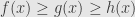 on a common domain containing a neighborhood of
  , and if
  , then the limit of at exists and is also equal to
  . Given any sequence
  converging to , our hypothesis tells us that
  . Given any neighborhood of ,
  and
and  are both within the neighborhood for sufficiently large
  , and then so will
  be in the neighborhood. Thus the image of the sequence under is “squeezed” between the images under and
  , and converges to as well.
These rules for limits suffice to calculate almost all the limits that we care about without having to mess around with the raw definitions. In fact, many calculus classes these days only skim the definition if they mention it at all. We can more or less get away with this while we’re only dealing with a single real variable, but later on the full power of the definition comes in handy.
There’s one more situation I should be a little more explicit about. If we are given a function on some domain and we want to find its limit at a border point (which includes the case of a single-point hole in the domain) and we can extend the function to a continuous function  on a larger domain
  which contains a neighborhood of the point in question, then
  . Indeed, given any sequence converging to we have
  (since they agree on ), and the limit of is just its value at . This extends what we did before to handle the case of
  at
at  , and similar situations will come up over and over in the future.
December 20, 2007 -
Posted by John Armstrong |
Analysis, Calculus


[…] Laws of Differentiation Just like we had the laws of limits we have a collection of rules to help us calculate derivatives. Let’s start with the most […]
Pingback by Algebraic Laws of Differentiation « The Unapologetic Mathematician | December 26, 2007 |
[…] some cases establish the continuity of simple functions (like coordinate projections) and then use limit laws to build up a larger class. But this approach fails for functions superficially similar to the […]
Pingback by Multivariable Limits « The Unapologetic Mathematician | September 17, 2009 |
i would luv 2 recieve questions
Questions about what?