The Jacobian

Now that we’ve used exterior algebras to come to terms with parallelepipeds and their transformations, let’s come back to apply these ideas to the calculus.

We’ll focus on a differentiable function , where is itself some open region in . That is, if we pick a basis and coordinates of , then the function is a vector-valued function of real variables with components . The differential, then, is itself a vector-valued function whose components are the differentials of the component functions: . We can write these differentials out in terms of partial derivatives:

Just like we said when discussing the chain rule, the differential at the point defines a linear transformation from the -dimensional space of displacement vectors at to the -dimensional space of displacement vectors at , and the matrix entries with respect to the given basis are given by the partial derivatives.

It is this transformation that we will refer to as the Jacobian, or the Jacobian transformation. Alternately, sometimes the representing matrix is referred to as the Jacobian, or the Jacobian matrix. Since this matrix is square, we can calculate its determinant, which is also referred to as the Jacobian, or the Jacobian determinant. I’ll try to be clear which I mean, but often the specific referent of “Jacobian” must be sussed out from context.

So, in light of our recent discussion, what does the Jacobian determinant mean? Well, imagine starting with a -dimensional parallelepiped at the point , with one side in each of the basis directions, and positively oriented. That is, it consists of the points with in the interval for some fixed . We’ll assume for the moment that this whole region lands within the region . It should be clear that this parallelepiped is represented by the wedge

which clearly has volume given by the product of all the .

Now the function sends this cube to a sort of curvy parallelepiped, consisting of the points , with each in the interval , and this image will have some volume. Unfortunately, we have no idea as yet how to measure such a volume. But we might be able to approximate it. Instead of using the actual curvy parallelepiped, we’ll build a new one. And if the are small enough, it will be more or less the same set of points, with the same volume. Or at least close enough for our purposes. We’ll replace the curved path defined by

by the displacement vector between the two endpoints:

and use these new vectors to build a new parallelepiped

But this is still an awkward volume to work with. However, we can use the differential to approximate each of these differences

with no summation here on the index .

Now we can easily calculate the volume of this parallelepiped, represented by the wedge

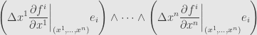
which can be rewritten as

which clearly has a volume of — the volume of the original parallelepiped — times the Jacobian determinant. That is, the Jacobian determinant at estimates the factor by which the function expands small volumes near that point. Or it tells us that locally reverses the orientation of small regions near the point if the Jacobian determinant is negative.