Proving the Classification Theorem I
This week, we will prove the classification theorem for root systems. The proof consist of a long series of steps, and we’ll split it up over a number of posts.
Our strategy is to determine which Coxeter graphs can arise from actual root systems, and then see what Dynkin diagrams we can get. Since Coxeter graphs ignore relative lengths of roots, we will start by just working with unit vectors whose pairwise angles are described by the Coxeter graph.
So, for the time being we make the following assumptions: 


We construct a Coxeter graph 
- If we remove some of the vectors from an admissible set, then the remaining vectors still form an admissible set. The Coxeter graph of the new set is obtained from that of the old one by removing the vertices corresponding to the removed vectors and all their incident edges.
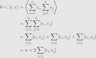
- The number of pairs of vertices in
- The graph
This should be straightforward. The remaining vectors are still linearly independent, and they still have unit length. The angles between each pair are also unchanged. All we do is remove some vectors (vertices in the graph).
Let us define

Since the 

Now, for any pair 


Indeed, if we have a cycle of length
8 Comments »
Leave a comment
RSS Feeds


Hi – I think you missed out a minus sign in step two, near the end: 2\langle\epsilon_i,\epsilon_j\rangle\leq1.
Paul
Ah yes, thanks.
[…] Proving the Classification Theorem II We continue with the proof of the classification theorem that we started yesterday. […]
Pingback by Proving the Classification Theorem II « The Unapologetic Mathematician | February 23, 2010 |
Students love to have a Big Theorem at the end of the semester, from which mountaintop to survey the landscape that they have mastered. This classification result is such a theorem.
Well it’s not done yet. After proving what was stated on Friday, we have to actually show whether or not any of these possible diagrams actually do occur.
[…] continue with the proof of the classification theorem. The first two parts are here and […]
Pingback by Proving the Classification Theorem III « The Unapologetic Mathematician | February 25, 2010 |
[…] Theorem IV We continue proving the classification theorem. The first three parts are here, here, and […]
Pingback by Proving the Classification Theorem IV « The Unapologetic Mathematician | February 25, 2010 |
[…] Today we conclude the proof of the classification theorem. The first four parts of the proof are here, here, here, and […]
Pingback by Proving the Classification Theorem V « The Unapologetic Mathematician | February 26, 2010 |