Proving the Classification Theorem IV
We continue proving the classification theorem. The first three parts are here, here, and here.
- Any connected graph
takes one of the four following forms: a simple chain, the
graph, three simple chains joined at a central vertex, or a chain with exactly one double edge.
- The only possible Coxeter graphs with a double edge are those underlying the Dynkin diagrams
,
, and
.
This step largely consolidates what we’ve done to this point. Here are the four possible graphs:


The labels will help with later steps.
Step 5 told us that there’s only one connected graph that contains a triple edge. Similarly, if we had more than one double edge or triple vertex, then we must be able to find two of them connected by a simple chain. But that will violate step 7, and so we can only have one of these features either.


Here we’ll use the labels on the above graph. We define


As in step 6, we find that 
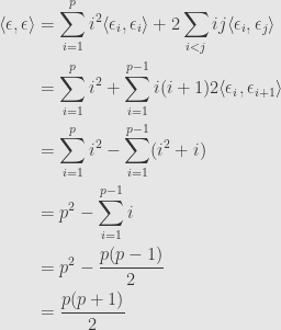
And similarly, 


Now we can use the Cauchy-Schwarz inequality to conclude that

where the inequality is strict, since 


We thus must have either 


5 Comments »
Leave a reply to Robert Cancel reply
RSS Feeds


Whoowee!
What program do you do your mathwriting in?
WordPress itself supports the writing. For these diagrams I’m using GeoGebra, while for big commutative diagrams I render them in TeXshop and cut/paste the images here.
Great work! I really enjoy these posts. You should consider joining up with Khan and making some videos of higher level maths.
You duplicated one line of the equations underneath “As in step 6…and so we calculate”.
Will you be going over how these tie in with polytopes?
Thanks, fixed it.
As it stands, I’m not planning on using the classification immediately. But it provides a nice break in the analysis work for a while.
[…] Proving the Classification Theorem V Today we conclude the proof of the classification theorem. The first four parts of the proof are here, here, here, and here. […]
Pingback by Proving the Classification Theorem V « The Unapologetic Mathematician | February 26, 2010 |