Integral Curves and Local Flows
Let  is a vector field on the manifold
  and let
  be any point in . Then I say there exists a neighborhood
  of , an interval
  around
  , and a differentiable map
 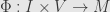 such that
for all  and
and  . These should look familiar, since they’re very similar to the conditions we wrote down for the flow of a differential equation.
It might help a bit to clarify that  is the inclusion
  of the canonical vector
  which points in the direction of increasing
  . That is,
 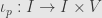 includes the interval
  into
into  “at the point “, and thus its derivative carries along its tangent bundle. At each point of an (oriented) interval there’s a canonical vector, and is the image of that vector.
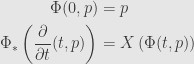
Further, take note that we can write the left side of our second condition as

The chain rule lets us combine these two outer derivatives into one:
![\displaystyle\left[\Phi\circ\iota_p\right]_*\left(\frac{d}{dt}(t)\right)](https://s0.wp.com/latex.php?latex=%5Cdisplaystyle%5Cleft%5B%5CPhi%5Ccirc%5Ciota_p%5Cright%5D_%2A%5Cleft%28%5Cfrac%7Bd%7D%7Bdt%7D%28t%29%5Cright%29&bg=e6e6e6&fg=333333&s=0&c=20201002)
But this is exactly how we defined the derivative of a curve! That is, we can write down a function  which satisfies
 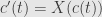 for every . We call such a curve an “integral curve” of the vector field
  , and when they’re collected together as in
  we call it a “local flow” of .
So how do we prove this? We just take local coordinates and use our good old existence theorem! Indeed, if  is a coordinate patch around then we can set
  ,
,  , and
, and

where the  are the components
  of relative to the given local coordinates.
Now our existence theorem tells us there is a neighborhood  of
of  , an interval around , and a map
  satisfying the conditions for a flow. Setting
  and
and  we find our local flow.
We can also do the same thing with our uniqueness theorem: if  and
and  are two integral curves of defined on the same interval , and if
  for some
  , then
  .
.
Thus we find the geometric meaning of that messy foray into analysis: a smooth vector field has a smooth local flow around every point, and integral curves of vector fields are unique.
May 28, 2011 -
Posted by John Armstrong |
Differential Topology, Topology


[…] a smooth vector field we know what it means for a curve to be an integral curve of . We even know how to find them by starting at a point and solving differential equations as […]
Pingback by The Maximal Flow of a Vector Field « The Unapologetic Mathematician | May 30, 2011 |
[…] we define a vector field by then is a flow for this vector field. Indeed, it’s a maximal flow, since it’s defined for all time at […]
Pingback by One-Parameter Groups « The Unapologetic Mathematician | May 31, 2011 |
[…] is a lot like an integral curve, with one slight distinction: in the case on an integral curve we also demand that the length of […]
Pingback by Integral Submanifolds « The Unapologetic Mathematician | June 30, 2011 |
[…] . So, given a point we may as well choose itself as the base-point. We know that we can choose an integral curve of through , and we also know […]
Pingback by Path-Independent 1-Forms are Exact « The Unapologetic Mathematician | December 15, 2011 |