How to Use the FToC

I’ll get back to deconstructing comics another time. For now, I want to push on with some actual mathematics.

After much blood, toil, tears, and sweat, we’ve proven the Fundamental Theorem of Calculus. So what do we do with it? The answer’s in this diagram:

This is sort of schematic rather than something we can interpret literally.

On the left we have real-valued functions — we’re being vague about their domains — and collections of “signed” points. We also have a way of pairing a function with a collection of points: evaluate the function at each point, and then add up all the values or their negatives, depending on the sign of the point. On the right we also have real-valued functions, but now we consider intervals of the real line. We have another way of pairing a function with an interval: integration!

At the top of the diagram, we can take a function and differentiate it to get back another function. At the bottom, we can take an interval and get a collection of signed points by moving to the boundary. The interval has the boundary points , where we consider to be “negatively signed”.

Now, what does the FToC tell us? If we start with a function in the upper left and an interval in the lower right, we have two ways of trying to pair them off. First, we could take the derivative of and then integrate it from to to get . On the other hand, we could take the boundary of the interval and add up the function values along the boundary to get . The FToC tells us that these two give us the same answer!

To write this in a diagram seems a little much, but keep the diagram in mind. We’ll come back to it later. For now, though, we can use it to understand how to use the FToC to handle integration.

Say we have a function and an interval , and we need to find . We’ve got these big, messy Riemann sums (or Darboux sums), and there’s a lot of work to compute the integral by hand. But notice that the integral is living on the right side of the diagram. If we could move it over to the left, we’d just have to evaluate a function twice and add up the results.

Moving the interval to the left of the diagram is easy: we can just read off the boundary. Moving the function is harder. What we need is to find an antiderivative so that . Then we move to the left of the diagram by switch attention from to . Then we can evaluate and get exactly the same value as the integral we set out to calculate. So if we want to find integrals, we’d better get good at finding antiderivatives!

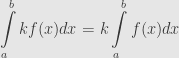
This has an immediate consequence. Our basic rules of antiderivatives carry over to give some basic rules for integration. In particular, we know that integrals play nicely with sums and scalar multiples: