Solving Equations with Gaussian Elimination

The row echelon form of a matrix isn’t unique, but it’s still useful for solving systems of linear equations. If we have a system written in matrix form as

$\displaystyle Ax=y$

then applying elementary row operations builds up a new matrix that we multiply on the left of both sides

$\displaystyle EAx=Ey$

If the new matrix $EA$ is in row echelon form, the resulting system of equations will be simple to solve.

A little more explicitly, this works because each of the equations is linear, and so each of the elementary row operations corresponds to some manipulation of the equations which gives rise to an equivalent system. for example, the order of the equations doesn’t matter, so swapping two of them (swapping two rows) doesn’t change the solution. Similarly, multiplying both sides of one equation by a nonzero number doesn’t change the solution to that equation, and so doesn’t change the solution of the system. Finally, adding two equations gives another valid equation. Since the three equations “overdetermine” the solution (they’re linearly dependent), we can drop one of the first two. The result is the same as a shear.

Since we’re just doing the same thing to the rows of the column vector $y$ as we are to the matrix $A$ , we may as well stack them beside each other. In this way, we get the “augmented matrix” of the system of equations. For example, we might have the system

$\displaystyle\begin{aligned}2x+y-z&=8\\-3x-y+2z&=-11\\-2x+y+2z&=-3\end{aligned}$

with the augmented matrix

$\displaystyle\begin{pmatrix}2&1&-1&8\\-3&-1&2&-11\\-2&1&2&-3\end{pmatrix}$

Then we can follow along our elimination from yesterday, applying the same steps to the system of equations. Foe example, if at this point we add the first and third equations we get $2y+z=5$ , “eliminating” the variable $x$ from the equation. We replace the third equation with this new, simpler equation, giving the effect of a shear just like we did yesterday.

At the end, we found the row echelon form

$\displaystyle\begin{pmatrix}2&1&-1&8\\{0}&\frac{1}{2}&\frac{1}{2}&1\\{0}&0&-1&1\end{pmatrix}$

which corresponds with the system

$\displaystyle\begin{aligned}2x+y-z&=8\\\frac{1}{2}y+\frac{1}{2}z&=1\\-z&=1\end{aligned}$

Now the equations are arranged like a ladder for us to climb up. First, we solve the bottom equation to find $z=-1$ . Then we can plug this into the next equation up to find $\frac{1}{2}y-\frac{1}{2}=1$ , which is easily solved to find $y=3$ . Then we plug both of these answers into the next equation up to find $2x+3+1=8$ , which is easily solved to find $x=2$ , and we’re done. In fact, this is why we use the word “echelon” — French for a rung of a ladder — to describe this form.

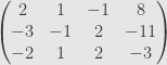
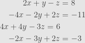
What about our other example from yesterday? This corresponds to a system of four equations with three unknowns, since we’re interpreting the last column as the column vector on the right side of the equation. The system is

$\displaystyle\begin{aligned}2x+y-z&=8\\-4x-2y+2z&=-11\\4x+4y-3z=6\\-2x-3y+2z&=-3\end{aligned}$

We convert this to an augmented matrix, put this matrix into row echelon form, and return it to the form of a system of equations to find

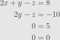
$\displaystyle\begin{aligned}2x+y-z&=8\\2y-z&=-10\\{0}&=5\\{0}&=0\end{aligned}$

The empty row on the bottom is fine, since it just tells us the tautology that $0=0$ . Unfortunately, the line above that contains the contradiction that $0=5$ . That is, whenever the row echelon form of a system of equations has a leading coefficient in the last column, that system is unsolvable. We don’t even need to climb the ladder to know that.

On the other hand, if we started with the system

$\displaystyle\begin{aligned}2x+y-z&=8\\-4x-2y+2z&=-16\\4x+4y-3z=6\\-2x-3y+2z&=2\end{aligned}$

and put it in row echelon form (do it yourself) we get

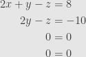
$\displaystyle\begin{aligned}2x+y-z&=8\\2y-z&=-10\\{0}&=0\\{0}&=0\end{aligned}$

Now we have no contradictions, but the system is underdetermined. Indeed, the rank is ${2}$ , so the kernel has dimension ${1}$ , and thus we’ll have one free parameter in our solution. It’s still easy to solve, though. We first find that $y=\frac{1}{2}z-5$ . Plugging this into the first equation we find $2x-\frac{1}{2}z-5=8$ , which is easily solved to find $x=\frac{1}{4}z-\frac{13}{2}$ .

So whether the system is exactly solvable, underdetermined, or contradictory, we can find whatever solutions may exist explicitly using a row echelon form.

September 2, 2009 - Posted by John Armstrong | Algebra, Linear Algebra

9 Comments »

I’ve been following this blog with Google Reader for a while, but it has been generally above my head, until last post when you shifted gears and went to the basics of linear algebra. I’m enjoying the reading. If you go from this material all the way to the topics from earlier I’ll probably get it this time around.

Comment by Robert Danhof | September 2, 2009 | Reply
Yes, I probably could have done this earlier, but I wanted to get does the idea of particular useful factorizations and things that were essentially basis-free before mucking about with something as basis heavy as elementary row operations and row echelon forms. This material is actually coming to the end of my work on linear algebra (after something like a full year’s worth of work on it). Soon I’ll be able to get into multivariable calculus.

Comment by John Armstrong | September 2, 2009 | Reply
[…] elimination we saved some steps by leaving pivoted rows alone. This was fine for the purposes of solving equations, where the point is just to eliminate progressively more and more variables in each equation. We […]

Pingback by Reduced Row Echelon Form « The Unapologetic Mathematician | September 3, 2009 | Reply
A few years ago I read some Numerical Methods lecture notes in Portuguese where a variant of the Gauss Elimination method was described. It is called partial pivoting and is intended to provide a greater numerical accuracy . First we exchange complete rows in the system augmented matrix $(A|B)$ so that the entry $a_{j,j}$ ( $1\le j\le n$ ) has the largest absolute value from all entries $a_{i,j}$ with $i\ge j$ and then proceed as in the normal Gauss elimination method applied to column $j$ .

For instance, starting with your first example

$\begin{pmatrix}2 & 1 & -1 & 8 \\ -3 & -1 & 2 & -11 \\ -2 & 1 & 2 & -3\end{pmatrix}$

we exchange rows 1 and 2 ( $\left\vert -3\right\vert >\left\vert 2\right\vert$ )

$\begin{pmatrix}-3 & -1 & 2 & -11 \\ 2 & 1 & -1 & 8 \\ -2 & 1 & 2 & -3\end{pmatrix}.$

Then we apply the pivoting method to column 1

$\begin{pmatrix}-3 & -1 & 2 & -11 \\ 0 & 1/3 & 1/3 & 2/3 \\ 0 & 5/3 & 2/3 & 13/3\end{pmatrix}.$

Now we exchange rows 2 and 3 ( $\left\vert \frac{5}{3}\right\vert >\left\vert \frac{1}{3}\right\vert$ )

$\begin{pmatrix}-3 & -1 & 2 & -11 \\ 0 & 5/3 & 2/3 & 13/3 \\ 0 & 1/3 & 1/3 & 2/3\end{pmatrix}$

and apply the normal method to column 2

$\begin{pmatrix}-3 & -1 & 2 & -11 \\ 0 & 5/3 & 2/3 & 13/3 \\ 0 & 0 & 1/5 & -1/5\end{pmatrix}.$

From here we get the system of equations

$-3x-y+2z=-11$

$\frac{5}{3}y+\frac{2}{3}z=\frac{13}{3}$

$\frac{1}{5}z=-\frac{1}{5}$

which we solve as before

$\frac{1}{5}z=-\frac{1}{5}\iff z=-1$

$\frac{5}{3}y+\frac{2}{3}\left( -1\right) =\frac{13}{3}\iff y=3$

$-3x-3+2\left( -1\right) =-11\iff x=2$ .

Comment by Américo Tavares | September 5, 2009 | Reply
Oh, sure Américo, there are more efficient algorithms, and optimizations on the basic algorithms, but I’m mainly going for what at UMD would be a 200-level linear algebra level approach to the subject, not a 460-level numerical analysis approach. But thanks for pointing that direction out.

Comment by John Armstrong | September 6, 2009 | Reply
Hello.
Could you comment on using the Inverse Matrix.
What if the matrix is singular in inhomogenous system?

Thanks.

Comment by Drazick | September 29, 2009 | Reply
Drazick

If it helps to the first part of your comment (I am not sure it does) here is an

Example: solve

$\left\{ \begin{array}{c}3x+4y+z=380 \\ 2x+4y+2z=400 \\ 6x+2y+2z=520\end{array}\right.$

and find the inverse matrix of

$A=\left(\begin{array}{ccc}3 & 4 & 1 \\2 & 4 & 2 \\6 & 2 & 2\end{array}\right)$ .

Let $i_1$ , $i_{2}$ and $i_{3}$ be the matrices

$i_{1}=\left( \begin{array}{c}1 \\ 0 \\ 0\end{array}\right)$

$i_{2}=\left(\begin{array}{c}0 \\ 1 \\ 0\end{array}\right)$

$i_{3}=\left( \begin{array}{c}0 \\ 0 \\ 1\end{array}\right)$

We form the three augmented matrices

$\left( A|i_{1}\right) =\left( \begin{array}{ccccc}3 & 4 & 1 & | & 1 \\ 2 & 4 & 2 & | & 0 \\ 6 & 2 & 2 & | & 0\end{array}\right)$

$\left( A|i_{2}\right) =\left( \begin{array}{ccccc}3 & 4 & 1 & | & 0 \\ 2 & 4 & 2 & | & 1 \\ 6 & 2 & 2 & | & 0\end{array}\right)$

$\left( A|i_{3}\right) =\left( \begin{array}{ccccc}3 & 4 & 1 & | & 0 \\ 2 & 4 & 2 & | & 0 \\ 6 & 2 & 2 & | & 1\end{array}\right)$

The application of the Gauss method with partial pivoting (see my comment No. 4 above) to the first matrix gives:

$\left( U|j_{1}\right) =\left( \begin{array}{ccccc}6 & 2 & 2 & | & 0 \\ 0 &\dfrac{10}{3} &\dfrac{4}{3} & | & 0 \\ 0 & 0 &-\dfrac{6}{5} & | & 1\end{array}\right) .$

To the second,

$\left( U|j_{2}\right) =\left( \begin{array}{ccccc}6 & 2 & 2 & | & 0 \\ 0 & \displaystyle\frac{10}{3} &\displaystyle\frac{4}{3} & | & 1 \\ 0 & 0 &\displaystyle-\frac{6}{5} & | &\displaystyle-\frac{9}{10}\end{array}\right) .$

And to the third one

$\left( U|j_{3}\right) =\left( \begin{array}{ccccc}6 & 2 & 2 & | & 1 \\ 0 & \displaystyle\frac{10}{3} &\displaystyle\frac{4}{3} & | & \displaystyle-\frac{1}{3} \\ 0 & 0 &\displaystyle-\frac{6}{5} & | &\displaystyle-\frac{2}{10}\end{array}\right)$

Solving

$U\cdot x=j_{1}$

$U\cdot y=j_{2}$

$U\cdot z=j_{3}$

we get

$x=\left( \begin{array}{c}1/6 \\ 1/3 \\ -5/6\end{array}\right)$

$y=\left( \begin{array}{c}-1/4 \\ 0 \\ 3/4\end{array}\right)$

$z=\left( \begin{array}{c}1/6 \\ 1/6 \\ 1/6\end{array}\right)$

that are the three columns of the inverse matrix $A^{-1}:$

$A^{-1}=\left( \begin{array}{ccc}1/6 & -1/4 & 1/6 \\ 1/3 & 0 & -1/6 \\ -5/6 & 3/4 & 1/6\end{array}\right)$

Comment by Américo Tavares | March 30, 2010 | Reply
wats the point or use of gaussian elimination?

Comment by bash | March 17, 2011 | Reply
Well for one thing it lets us solve systems of linear equations, as this post itself explains.

Comment by John Armstrong | March 17, 2011 | Reply

About this weblog

This is mainly an expository blath, with occasional high-level excursions, humorous observations, rants, and musings. The main-line exposition should be accessible to the “Generally Interested Lay Audience”, as long as you trace the links back towards the basics. Check the sidebar for specific topics (under “Categories”).

I’m in the process of tweaking some aspects of the site to make it easier to refer back to older topics, so try to make the best of it for now.

RSS Feeds

RSS - Posts
RSS - Comments
Feedback

Got something to say? Anonymous questions, comments, and suggestions at Formspring.me!
Subjects

Subjects
Archives

September 2009

M T W T F S S

1 2 3 4 5 6

7 8 9 10 11 12 13

14 15 16 17 18 19 20

21 22 23 24 25 26 27

28 29 30

« Aug Oct »
Search for:

The Unapologetic Mathematician

Mathematics for the interested outsider