Extrema with Constraints I
We can consider the problem of maximizing or minimizing a function, as we have been, but insisting that our solution satisfy some constraint.
For instance, we might have a function  to maximize, but we’re only concerned with unit-length vectors on
  . More generally, we’ll be concerned with constraints imposed by setting a function
  equal to zero. In the example, we might set
  . If we want to impose more conditions, we can make a vector-valued function with as many components as constraint functions we want to set equal to zero.
Now, we might be able to parameterize the collection of points satisfying  . In the example, we could use the usual parameterization of the sphere by latitude and longitude, writing

where I’ve used the physicists’ convention on the variables instead of the common one in multivariable calculus classes. Then we could plug these expressions for  ,
,  , and
, and  into our function
  , and get a composite function of the variables
  and
and  , which we can then attack with the tools from the last couple days, being careful about when we can and can’t trust Cauchy’s invariant rule, since the second differential can transform oddly.
Besides even that care that must be taken, it may not even be possible to parameterize the surface, or it may be extremely difficult. At least we do know that such a parameterization will often exist. Indeed, the implicit function theorem tells us that if we have  continuously differentiable constraint functions
  whose zeroes describe a collection of points in an
  -dimensional space
  , and the
  determinant

is nonzero at some point  satisfying
  , then we can “solve” these equations for the first variables as functions of the last
  . This gives us exactly such a parameterization, and in principle we could use it. But the calculations get amazingly painful.
Instead, we want to think about this problem another way. We want to consider a point is a point satisfying which has a neighborhood  so that for all
  satisfying we have
  . This does not say that there are no nearby points to
  where takes on larger values, but it does say that to reach any such point we must leave the region described by .
Now, let’s think about this sort of heuristically. As we look in various directions  from , some of them are tangent to the region described by . These are the directions satisfying
 =dg(a;v)=0](https://s0.wp.com/latex.php?latex=%5BD_vg%5D%28a%29%3Ddg%28a%3Bv%29%3D0&bg=e6e6e6&fg=333333&s=0&c=20201002) — where to first order the value of is not changing in the direction of . I say that in none of these directions can change (again, to first order) either. For if it did, either would increase in that direction or not. If it did, then we could find a path in the region where along which was increasing, contradicting our assertion that we’d have to leave the region for this to happen. But if decreased to first order, then it would increase to first order in the opposite direction, and we’d have the same problem. That is, we must have
— where to first order the value of is not changing in the direction of . I say that in none of these directions can change (again, to first order) either. For if it did, either would increase in that direction or not. If it did, then we could find a path in the region where along which was increasing, contradicting our assertion that we’d have to leave the region for this to happen. But if decreased to first order, then it would increase to first order in the opposite direction, and we’d have the same problem. That is, we must have  whenever
  . And so we find that
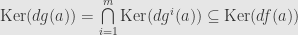
The kernel of  consists of all vectors orthogonal to the gradient vector
  , and the line it spans is the orthogonal complement to the kernel. Similarly, the kernel of
  consists of all vectors orthogonal to each of the gradient vectors
  , and is thus the orthogonal complement to the entire subspace they span. The kernel of is contained in the kernel of , and orthogonal complements are order-reversing, which means that must lie within the span of the . That is, there must be real numbers
  so that
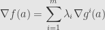
or, passing back to differentials

So in the presence of constraints we replace the condition  by this one. We call the “Lagrange multipliers”, and for every one of these variables we add to the system of equations, we also add the constraint equation
  , so we should still get an isolated collection of points.
Now, we reached this conclusion by a rather handwavy argument about being able to find increasing directions and so on within the region . This line of reasoning could possibly be firmed up, but we’ll find our proof next time in a slightly different approach.
November 25, 2009 -
Posted by John Armstrong |
Analysis, Calculus


Is there any systematic technique to the problem of maximizing or minimizing a function subject to constraints if one of the variables (I denote ) instead of being continuous is discrete both in the function
  and in the constraints
  ?
?
To me a naive approach that I describe briefly seems to be:
(1) start by fixing and get a “first solution” depending on
  .
.
(2) Then assuming were continuous find an “artificial solution”, let’s say
  .
.
(3) Finally compute the values of at the nearest integers to
  and choose according to the (maximizing or minimizing) type of problem .
This procedure is feasible in particular cases and the solution is near to the optimized one but I suspect that in general there is no guaranty.
I’m not sure in general, Américo. What I’d suggest is Hancock’s Theory of Maxima and Minima, which I know of mainly because it contains an analytic method to distinguish maxima and minima subject to constraints (like the second derivative test).
Many thanks, John.
[…] with Constraints II As we said last time, we have an idea for a necessary condition for finding local extrema subject to constraints of a […]
Pingback by Extrema with Constraints II « The Unapologetic Mathematician | November 27, 2009 |