Inner Products on 1-Forms
Our next step after using a metric to define an inner product on the module  of vector spaces over the ring
  of smooth functions is to flip it around to the module
  of
of  -forms. The nice thing is that the hard part is already done. All we really need to do is define an inner product on the cotangent space
  ; then the extension to -forms is exactly like extending from inner products on each tangent space to an inner product on vector fields.
And really this construction is just a special case of a more general one. Let’s say that  is an inner product on a vector space
  . As we mentioned when discussing adjoint transformations, this gives us an isomorphism from to its dual space
  . That is, when we have a metric floating around we have a canonical way of identifying tangent vectors in
  with cotangent vectors in
  .
.
Everything is perfectly well-defined at this point, but let’s consider this a bit more explicitly. Say that  is a basis of . We automatically have a dual basis
  defined by
  , even before defining the metric. So if the inner product
  defines a mapping
  , what does it look like with respect to these bases? It takes the vector
  and sends it to a linear functional whose value at
  is
is  . Since we get a number at each point
  , we will also write this as a function
  That is, we can break the image of out as the linear combination
What about a vector with components  ? We easily calculate

So  is the matrix of this transformation. The fact that both indices on the bottom tells us that we are moving from vectors to covectors.
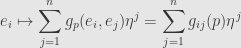
The same sort of reasoning can be applied to the inner product on the dual space. If we write it again by , then we get another matrix:

which tells us how to send a basis covector  to a vector:

and thus we can calculate the image of any covector with components  :
:

But these are supposed to be inverses to each other! Thus we can send a vector  to a covector and back:
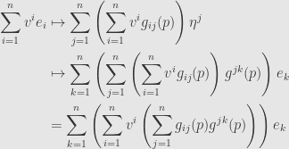
If this is to be the original vector back, the coefficient of  must be
  , which means the inner sum — the matrix product of and
  — must be the Kronecker delta. That is, must be the right matrix inverse of .
Similarly, if we start with a covector we will find that  must be the left matrix inverse of
  . Since it’s a left and a right inverse, it must be the inverse; in particular, must be invertible, which is equivalent to the assumption that is nondegenerate! It also means that we can always find the matrix of the inner product on the dual space in terms of the dual basis, assuming we have the matrix of the inner product on the original space.
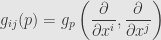
And to return to differential geometry, let’s say we have a coordinate patch  . We get a basis of coordinate vector fields, which let us define the matrix-valued function
This much we calculate from the metric we are given by assumption. But then we can invert the matrix at each point to get another one:

where this is how we define the inner product on covectors. Of course, the situation is entirely symmetric, and if we’d started with a symmetric tensor field of type  that defined an inner product at each point, we could flip it over to get a metric.
October 1, 2011 -
Posted by John Armstrong |
Differential Geometry, Geometry


[…] that we’ve defined inner products on -forms we can define them on forms for all other . In fact, our construction will not depend on […]
Pingback by Inner Products on Differential Forms « The Unapologetic Mathematician | October 4, 2011 |
[…] Now, we already have something else floating around in our discussion: the metric tensor . When we pick coordinates we get a matrix-valued function: […]
Pingback by The Hodge Star on Differential Forms « The Unapologetic Mathematician | October 6, 2011 |
[…] Armstrong: (Pseudo)-Riemannian Metrics, Isometries, Inner Products on 1-Forms, The Hodge Star in Coordinates, The Hodge Star on Differential Forms, Inner Products on […]
Pingback by Thirteenth Linkfest | October 8, 2011 |
[…] we know that and are inverse matrices. And so we get the canonical volume […]
Pingback by A Hodge Star Example « The Unapologetic Mathematician | October 11, 2011 |
[…] Inner Products on 1-Forms (unapologetic.wordpress.com) […]