Charge Distibutions
The superposition principle for the electric field extends to the realm of continuous distributions, with the sum replaced by an appropriate integral.
For example, let’s say we have a curve ![c:[0,1]\to\mathbb{R}^3](https://s0.wp.com/latex.php?latex=c%3A%5B0%2C1%5D%5Cto%5Cmathbb%7BR%7D%5E3&bg=e6e6e6&fg=333333&s=0&c=20201002) , and along this curve we have a charge. It makes sense to measure the charge in units per unit of distance, like coulombs per meter. We can even let it vary from point to point, getting a function
, and along this curve we have a charge. It makes sense to measure the charge in units per unit of distance, like coulombs per meter. We can even let it vary from point to point, getting a function  describing the charge per unit length near the point with parameter
  . To be a little more explicit, if
  is the “line element” that measures a tiny bit of distance near the point
  , then
  measures a little bit of charge near that point.
We can now use the Coulomb law to see what electric field this tiny bit of charge creates at a point with position vector  :
:

since the displacement vector from to is  . Now we can take this “differential electric field” and integrate it over the curve, adding up all the tiny contributions to the field at made by all the tiny bits of charge along the curve.
As an example, let’s consider an infinite line of charge along the  axis with a constant charge density of
  ; a piece of the line of length
  will have charge
  . Admittedly, this is not a finite-length curve like above, but the same principle applies. We set
  , so
, so  and
and  .
.
Geometric considerations tell us that the electric field generated by the line at a point is contained in the same plane that contains the line and the point. We can also tell that the field points directly perpendicular to the line; if  then the vertical component induced by the chunk at
  is cancelled out by the component induced by the chunk at
  . Indeed, we can check that the first gives us

while the second gives us

and the vertical components of these two exactly cancel each other out.
All that remains is to calculate the horizontal component. Without loss of generality we can consider the point  , and we must calculate the
  -component of the electric field by taking the integral
We need an antiderivative of the integrand  , and it turns out that
 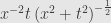 fits the bill. Indeed, we check:

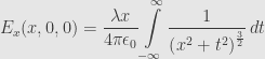
as asserted. Thus we continue the integration:
![\displaystyle\begin{aligned}E_x(x,0,0)&=\frac{\lambda x}{4\pi\epsilon_0}\int\limits_{-\infty}^\infty\frac{1}{\left(x^2+t^2\right)^\frac{3}{2}}\,dt\\&=\frac{\lambda x}{4\pi\epsilon_0}\lim\limits_{a,b\to\infty}\left[\frac{t}{x^2\sqrt{x^2+t^2}}\right]_{-a}^b\\&=\frac{\lambda}{4\pi\epsilon_0x}\lim\limits_{a,b\to\infty}\left(\frac{b}{\sqrt{x^2+b^2}}-\frac{-a}{\sqrt{x^2+a^2}}\right)\\&=\frac{\lambda}{4\pi\epsilon_0x}(1+1)\\&=\frac{1}{2\pi\epsilon_0}\frac{\lambda}{x}\end{aligned}](https://s0.wp.com/latex.php?latex=%5Cdisplaystyle%5Cbegin%7Baligned%7DE_x%28x%2C0%2C0%29%26%3D%5Cfrac%7B%5Clambda+x%7D%7B4%5Cpi%5Cepsilon_0%7D%5Cint%5Climits_%7B-%5Cinfty%7D%5E%5Cinfty%5Cfrac%7B1%7D%7B%5Cleft%28x%5E2%2Bt%5E2%5Cright%29%5E%5Cfrac%7B3%7D%7B2%7D%7D%5C%2Cdt%5C%5C%26%3D%5Cfrac%7B%5Clambda+x%7D%7B4%5Cpi%5Cepsilon_0%7D%5Clim%5Climits_%7Ba%2Cb%5Cto%5Cinfty%7D%5Cleft%5B%5Cfrac%7Bt%7D%7Bx%5E2%5Csqrt%7Bx%5E2%2Bt%5E2%7D%7D%5Cright%5D_%7B-a%7D%5Eb%5C%5C%26%3D%5Cfrac%7B%5Clambda%7D%7B4%5Cpi%5Cepsilon_0x%7D%5Clim%5Climits_%7Ba%2Cb%5Cto%5Cinfty%7D%5Cleft%28%5Cfrac%7Bb%7D%7B%5Csqrt%7Bx%5E2%2Bb%5E2%7D%7D-%5Cfrac%7B-a%7D%7B%5Csqrt%7Bx%5E2%2Ba%5E2%7D%7D%5Cright%29%5C%5C%26%3D%5Cfrac%7B%5Clambda%7D%7B4%5Cpi%5Cepsilon_0x%7D%281%2B1%29%5C%5C%26%3D%5Cfrac%7B1%7D%7B2%5Cpi%5Cepsilon_0%7D%5Cfrac%7B%5Clambda%7D%7Bx%7D%5Cend%7Baligned%7D&bg=e6e6e6&fg=333333&s=0&c=20201002)
which is a nice, tidy value. More generally, we find

pointing directly away from the (positively) charged line, neither up nor down, and falling off in magnitude as the first power of the distance from the line.
January 6, 2012 -
Posted by John Armstrong |
Electromagnetism, Mathematical Physics


[…] A better example is a current flowing along a curve (without boundary) with a (constant) charge density of . It’s possible to carry through the discussion with a variable charge density, but then […]
Pingback by Currents « The Unapologetic Mathematician | January 7, 2012 |
missing absolute value around the curve derivative at the end of paragraph 1
Thanks, fixing.
[…] future, if only to get the practice. We’ll start with a “charged ring” which is a charge distribution on a circle. Specifically, we may as well consider the circle of radius in the – plane: . If the […]
Pingback by Charged Rings and Planes « The Unapologetic Mathematician | January 10, 2012 |
[…] we replace our point charge with a charge distribution over some region of . This may be concentrated on some surfaces, or on curves, or at points, or […]
Pingback by Gauss’ Law « The Unapologetic Mathematician | January 11, 2012 |
[…] let’s see where we are. There is such a thing as charge, and there is such a thing as current, which often — but not always — arises from […]
Pingback by Maxwell’s Equations « The Unapologetic Mathematician | February 1, 2012 |
“falling off in magnitude”
I’m such a nitpicker.
Don’t worry about it, Hunt; I’m glad someone caught it. If we didn’t fix all the little mistakes we’d be physicists.