Plane Waves
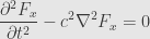
We’ve derived a “wave equation” from Maxwell’s equations, but it’s not clear what it means, or even why this is called a wave equation. Let’s consider the abstracted form, which both electric and magnetic fields satisfy:

where  is the “Laplacian” operator, defined on scalar functions by taking the gradient followed by the divergence, and extended linearly to vector fields. If we have a Cartesian coordinate system — and remember we’re working in good, old
  so it’s possible to pick just such coordinates, albeit not canonically — we can write
where  is the
  -component of
  , and a similar equation holds for the
  and
and  components as well. We can also write out the Laplacian in terms of coordinate derivatives:
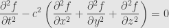
Let’s simplify further to just consider functions that depend on and  , and which are constant in the and directions:
![\displaystyle\frac{\partial^2f}{\partial t^2}-c^2\frac{\partial^2f}{\partial x^2}=\left[\frac{\partial^2}{\partial t^2}-c^2\frac{\partial^2}{\partial x^2}\right]f=0](https://s0.wp.com/latex.php?latex=%5Cdisplaystyle%5Cfrac%7B%5Cpartial%5E2f%7D%7B%5Cpartial+t%5E2%7D-c%5E2%5Cfrac%7B%5Cpartial%5E2f%7D%7B%5Cpartial+x%5E2%7D%3D%5Cleft%5B%5Cfrac%7B%5Cpartial%5E2%7D%7B%5Cpartial+t%5E2%7D-c%5E2%5Cfrac%7B%5Cpartial%5E2%7D%7B%5Cpartial+x%5E2%7D%5Cright%5Df%3D0&bg=e6e6e6&fg=333333&s=0&c=20201002)
We can take this big operator and “factor” it:
![\displaystyle\left[\left(\frac{\partial}{\partial t}+c\frac{\partial}{\partial x}\right)\left(\frac{\partial}{\partial t}-c\frac{\partial}{\partial x}\right)\right]f=0](https://s0.wp.com/latex.php?latex=%5Cdisplaystyle%5Cleft%5B%5Cleft%28%5Cfrac%7B%5Cpartial%7D%7B%5Cpartial+t%7D%2Bc%5Cfrac%7B%5Cpartial%7D%7B%5Cpartial+x%7D%5Cright%29%5Cleft%28%5Cfrac%7B%5Cpartial%7D%7B%5Cpartial+t%7D-c%5Cfrac%7B%5Cpartial%7D%7B%5Cpartial+x%7D%5Cright%29%5Cright%5Df%3D0&bg=e6e6e6&fg=333333&s=0&c=20201002)
Any function which either “factor” sends to zero will be a solution of the whole equation. We find solutions like
![\displaystyle\begin{aligned}\left[\frac{\partial}{\partial t}+c\frac{\partial}{\partial x}\right]A(x-ct)&=A'(x-ct)\frac{\partial(x-ct)}{\partial t}+cA'(x-ct)\frac{\partial(x-ct)}{\partial x}\\&=A'(x-ct)(-c+c)=0\\\left[\frac{\partial}{\partial t}-c\frac{\partial}{\partial x}\right]B(x+ct)&=B'(x+ct)\frac{\partial(x+ct)}{\partial t}-cB'(x+ct)\frac{\partial(x+ct)}{\partial x}\\&=B'(x+ct)(c-c)=0\end{aligned}](https://s0.wp.com/latex.php?latex=%5Cdisplaystyle%5Cbegin%7Baligned%7D%5Cleft%5B%5Cfrac%7B%5Cpartial%7D%7B%5Cpartial+t%7D%2Bc%5Cfrac%7B%5Cpartial%7D%7B%5Cpartial+x%7D%5Cright%5DA%28x-ct%29%26%3DA%27%28x-ct%29%5Cfrac%7B%5Cpartial%28x-ct%29%7D%7B%5Cpartial+t%7D%2BcA%27%28x-ct%29%5Cfrac%7B%5Cpartial%28x-ct%29%7D%7B%5Cpartial+x%7D%5C%5C%26%3DA%27%28x-ct%29%28-c%2Bc%29%3D0%5C%5C%5Cleft%5B%5Cfrac%7B%5Cpartial%7D%7B%5Cpartial+t%7D-c%5Cfrac%7B%5Cpartial%7D%7B%5Cpartial+x%7D%5Cright%5DB%28x%2Bct%29%26%3DB%27%28x%2Bct%29%5Cfrac%7B%5Cpartial%28x%2Bct%29%7D%7B%5Cpartial+t%7D-cB%27%28x%2Bct%29%5Cfrac%7B%5Cpartial%28x%2Bct%29%7D%7B%5Cpartial+x%7D%5C%5C%26%3DB%27%28x%2Bct%29%28c-c%29%3D0%5Cend%7Baligned%7D&bg=e6e6e6&fg=333333&s=0&c=20201002)
where  and
and  are pretty much any function that’s at least mildly well-behaved.
We call solutions of the first form “right-moving”, for if we view as time and watch as it increases, the “shape” of  stays the same; it just moves in the increasing direction. That is, at time
  we see the same thing at that we saw at
  —
—  units to the left — at time
  . Similarly, we call solutions of the second form “left-moving”. In each family, solutions propagate at a rate of
  , which was the constant from our original equation. Any solution of this simplified, one-dimensional wave equation will be the sum of a right-moving and a left-moving term.
More generally, for the three-dimensional version we have “plane-wave” solutions propagating in any given direction we want. We could do a big, messy calculation, but note that if  is any unit vector, we can pick a Cartesian coordinate system where is the unit vector in the direction, in which case we’re back to the right-moving solutions from above. And of course there’s no reason we can’t let be a vector-valued function. Such a solution looks like

The bigger is, the further in the direction the position vector  must extend to compensate; the shape
  stays the same, but moves in the direction of with a velocity of .
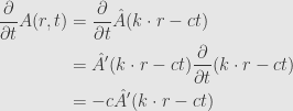
It will be helpful to work out some of the basic derivatives of such solutions. Time is easy:
Spatial derivatives are a little trickier. We pick a Cartesian coordinate system to write:

We don’t really want to depend on coordinates, so luckily it’s easy enough to figure out:

which will make our lives much easier to have worked out in advance.
February 8, 2012 -
Posted by John Armstrong |
Analysis, Differential Equations


[…] we’ve derived the wave equation from Maxwell’s equations, and we have worked out the plane-wave solutions. But there’s more to Maxwell’s equations than just the wave equation. Still, […]
Pingback by The Propagation Velocity of Electromagnetic Waves « The Unapologetic Mathematician | February 9, 2012 |
[…] look at another property of our plane wave solutions of Maxwell’s equations. Specifically, we’ll assume that the electric and magnetic […]
Pingback by Polarization of Electromagnetic Waves « The Unapologetic Mathematician | February 10, 2012 |
[…] Plane Waves « The Unapologetic MathematicianFeb 8, 2012 … Plane Waves. We’ve derived a “wave equation” from Maxwell’s equations, but it’s not clear what it means, or even why this is called a wave … […]
Pingback by Plane wave | Ajaygoud | April 2, 2012 |