The Unapologetic Mathematician

Mathematics for the interested outsider

The Faraday Field

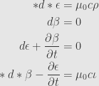
Now that we’ve seen that we can use the speed of light as a conversion factor to put time and space measurements on an equal footing, let’s actually do it to Maxwell’s equations. We start by moving the time derivatives over on the same side as all the space derivatives:

\displaystyle\begin{aligned}*d*\epsilon&=\mu_0c\rho\\d\beta&=0\\d\epsilon+\frac{\partial\beta}{\partial t}&=0\\{}*d*\beta-\frac{\partial\epsilon}{\partial t}&=\mu_0c\iota\end{aligned}

The exterior derivatives here written as d comprise the derivatives in all the spatial directions. If we pick coordinates x, y, and z, then we can write the third equation as three component equations that each look something like

\displaystyle\frac{\partial\epsilon_x}{\partial y}dy\wedge dx+\frac{\partial\epsilon_y}{\partial x}dx\wedge dy+\frac{\partial\beta_x}{\partial t}dx\wedge dy=\left(\frac{\partial\epsilon_y}{\partial x}-\frac{\partial\epsilon_x}{\partial y}+\frac{\partial\beta_z}{\partial t}\right)dx\wedge dy=0

This doesn’t look right at all! We’ve got a partial derivative with respect to t floating around, but I see no corresponding dt. So if we’re going to move to a four-dimensional spacetime and still use exterior derivatives, we can pick up dt terms from the time derivative of \beta. But for the others to cancel off, they already need to have a dt around in the first place. That is, we don’t actually have an electric 1-form:

\displaystyle\epsilon=\epsilon_xdx+\epsilon_ydy+\epsilon_zdz

In truth we have an electric 2-form:

\displaystyle\epsilon=\epsilon_xdx\wedge dt+\epsilon_ydy\wedge dt+\epsilon_zdz\wedge dt

Now, what does this mean for the exterior derivative d\epsilon?

\displaystyle\begin{aligned}d\epsilon=&\frac{\partial\epsilon_x}{\partial y}dy\wedge dx\wedge dt+\frac{\partial\epsilon_x}{\partial z}dz\wedge dx\wedge dt\\&+\frac{\partial\epsilon_y}{\partial x}dx\wedge dy\wedge dt+\frac{\partial\epsilon_y}{\partial z}dz\wedge dy\wedge dt\\&+\frac{\partial\epsilon_z}{\partial x}dx\wedge dz\wedge dt+\frac{\partial\epsilon_z}{\partial y}dy\wedge dz\wedge dt\\=&\left(\frac{\partial\epsilon_y}{\partial x}-\frac{\partial\epsilon_x}{\partial y}\right)dx\wedge dy\wedge dt\\&+\left(\frac{\partial\epsilon_x}{\partial z}-\frac{\partial\epsilon_z}{\partial x}\right)dz\wedge dx\wedge dt\\&+\left(\frac{\partial\epsilon_z}{\partial y}-\frac{\partial\epsilon_y}{\partial z}\right)dy\wedge dz\wedge dt\end{aligned}

Nothing has really changed, except now there’s an extra factor of dt at the end of everything.

What happens to the exterior derivative of \beta now that we’re using t as another coordinate? Well, in components we write:

\displaystyle\beta=\beta_xdy\wedge dz+\beta_ydz\wedge dx+\beta_zdx\wedge dy

and thus we calculate:

\displaystyle\begin{aligned}d\beta=&\frac{\partial\beta_x}{\partial x}dx\wedge dy\wedge dz+\frac{\partial\beta_x}{\partial t}dt\wedge dy\wedge dz\\&+\frac{\partial\beta_y}{\partial y}dy\wedge dz\wedge dx+\frac{\partial\beta_y}{\partial t}dt\wedge dz\wedge dx\\&+\frac{\partial\beta_z}{\partial z}dz\wedge dx\wedge dy+\frac{\partial\beta_z}{\partial t}dt\wedge dx\wedge dy\\=&\left(\frac{\partial\beta_x}{\partial x}+\frac{\partial\beta_y}{\partial y}+\frac{\partial\beta_z}{\partial z}\right)dx\wedge dy\wedge dz\\&+\frac{\partial\beta_z}{\partial t}dx\wedge dy\wedge dt+\frac{\partial\beta_y}{\partial t}dz\wedge dx\wedge dt+\frac{\partial\beta_x}{\partial t}dy\wedge dz\wedge dt\end{aligned}

Now the first part of this is just the old, three-dimensional exterior derivative of \beta, corresponding to the divergence. The second of Maxwell’s equations says that it’s zero. And the other part of this is the time derivative of \beta, but with an extra factor of dt.

So let’s take the 2-form \epsilon and the 2-form \beta and put them together:

\displaystyle\begin{aligned}d(\epsilon+\beta)=&d\epsilon+d\beta\\=&\left(\frac{\partial\beta_x}{\partial x}+\frac{\partial\beta_y}{\partial y}+\frac{\partial\beta_z}{\partial z}\right)dx\wedge dy\wedge dz\\&+\left(\frac{\partial\epsilon_y}{\partial x}-\frac{\partial\epsilon_x}{\partial y}+\frac{\partial\beta_z}{\partial t}\right)dx\wedge dy\wedge dt\\&+\left(\frac{\partial\epsilon_x}{\partial z}-\frac{\partial\epsilon_z}{\partial x}+\frac{\partial\beta_y}{\partial t}\right)dz\wedge dx\wedge dt\\&+\left(\frac{\partial\epsilon_z}{\partial y}-\frac{\partial\epsilon_y}{\partial z}+\frac{\partial\beta_x}{\partial t}\right)dy\wedge dz\wedge dt\end{aligned}

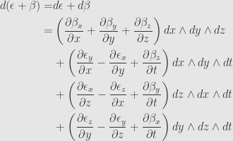
The first term vanishes because of the second of Maxwell’s equations, and the rest all vanish because they’re the components of the third of Maxwell’s equations. That is, the second and third of Maxwell’s equations are both subsumed in this one four-dimensional equation.

When we rewrite the electric and magnetic fields as 2-forms like this, their sum is called the “Faraday field” F. The second and third of Maxwell’s equations are equivalent to the single assertion that dF=0.

March 6, 2012 - Posted by | Electromagnetism, Mathematical Physics

4 Comments »

  1. […] we push ahead with the Faraday field in hand, we need to properly define the Hodge star in our four-dimensional space, and we need a […]

    Pingback by Minkowski Space « The Unapologetic Mathematician | March 7, 2012 | Reply

  2. that’s help me, thank for your faraday explanation

    Comment by arif | April 3, 2012 | Reply

  3. […] a vacuum we just have the electromagnetic fields and no charge or current distribution. We use the Faraday field to write down the […]

    Pingback by The Higgs Mechanism part 2: Examples of Lagrangian Field Equations « The Unapologetic Mathematician | July 17, 2012 | Reply

  4. […] — if we expand out as if it’s the Faraday field into “electric” and “magnetic” fields — give us Gauss’ and […]

    Pingback by The Higgs Mechanism part 3: Gauge Symmetries « The Unapologetic Mathematician | July 18, 2012 | Reply


Leave a comment