The Higgs Mechanism part 1: Lagrangians

This is part one of a four-part discussion of the idea behind how the Higgs field does its thing.

Wow, about six months’ hiatus as other parts of my life have taken precedence. But I drag myself slightly out of retirement to try to fill a big gap in the physics blogosphere: how the Higgs mechanism works.

There’s a lot of news about this nowadays, since the Large Hadron Collider has announced evidence of a “Higgs-like” particle. As a quick explanation of that, I use an analogy I made up on Twitter: “If Mirror-Spock exists, he has a goatee. We have found a man with a goatee. We do not yet know if he is Mirror-Spock.”

So, what is the Higgs boson? Well, it’s the particle expression of the Higgs field. That doesn’t explain anything, so we go one step further. What is the Higgs field? It’s the (conjectured) thing that gives some other particles (some of their) mass, in certain situations where normally we wouldn’t expect there to be any mass. And then there’s hand-waving about something like the ether that particles have to push through or shag carpet that they have to rub against that slows them down and hey, mass. Which doesn’t really explain anything, but sort of sounds like it might and so people nod sagely and then either forget about it all or spin their misconceptions into a new wave of Dancing Wu-Li Masters.

I think we can do better, at least for the science geeks out there who are actually interested and not allergic to a little math.

A couple warnings and comments before we begin. First off: I’m not going to go through this in my usual depth because I want to cram it into just three posts, albeit longer ones than usual, even though what I will say touches on all sorts of insanely cool mathematics that disappointingly few people see put together like this. Second: Ironically, that seems to include a lot of the physicists, who are generally more concerned with making predictions than with understanding how the underlying theory connects to everything else and it’s totally fine, honestly, that they’re interested in different aspects than I am. But I’m going to make a relatively superficial pass over describing the theory as physicists talk about it rather than go into those underlying structures. Lastly: I’m not going to describe the actual Higgs particle or field as they exist in the Standard Model; that would require quantum field theory and all sorts of messy stuff like that, when it turns out that the basic idea already shows up in classical field theory, which is a lot easier to explain. Even within classical field theory I’m going to restrict myself to a simpler example of the sort of thing that happens. Because reasons.

That all said, let’s dive in with Lagrangian mechanics. This is a subject that you probably never heard about unless you were a physics major or maybe a math major. Basically, Newtonian mechanics works off of the three laws that were probably drilled into your head by the end of high school science classes:

Newton’s Laws of Motion
1. An object at rest tends to stay at rest; an object in motion tends to stay in that motion.
2. Force applied to an object is proportional to the acceleration that object experiences. The constant of proportionality is the object’s mass.
3. Every action comes paired with an equal and opposite reaction.

It’s the second one that gets the most use since we can write it down in a formula: . And for most forces we’re interested in the force is a conservative vector field, meaning that it’s the (negative) gradient (fancy word for “derivative” that comes up in more than one dimension) of a potential energy function: . What this means is that things like to move in the direction that potential energy decreases, and they “feel a force” pushing them in that direction. Upshot for Newton: .

Lagrangian mechanics comes at this same formula with a different explanation: objects like to move along paths that (locally) minimize some quantity called “action”. This principle unifies the usual topics of high school Newtonian physics with things like optics where we say that light likes to move along the shortest path between two points. Indeed, the “action” for light rays is just the distance they travel! This also explains things like “the angle of incidence equals the angle of reflection”; if you look at all paths between two points that bounce off of a mirror, the one that satisfies this property has the shortest length, making it a local minimum for the action.

Let’s set this up for a body moving around in some potential field to show you how it works. The action of a suggested path — the body is at the point at time over a time interval is:

where is the velocity vector of the particle, is the square of its length, and is a potential function depending only on the position of the particle. Don’t worry: there’s a big scary integral here, but we aren’t going to actually do any integration.

The function on the inside of the integral is called the Lagrangian function, and we calculate the action of the path by integrating the Langrangian over the time interval we’re concerned with. We write this as with square brackets to emphasize that this is a “functional” that takes a function and gives a number back. Of course, as mathematicians there’s really nothing inherently special about functions taking functions as arguments, but for beginners it helps keep things straight.

Now, what happens if we “wiggle” the path a bit? What if we calculate the action of , where is some “small” function called the “variation” of ? We calculate:

Taking the derivative is linear, so we see that ; “the variation of the derivative is the derivative of the variation”. Plugging this in:

where we’ve thrown away terms involving second and higher powers of ; the variation is small, so the square (and cube, and …) is negligible. So what’s the difference between this and ? What’s the variation of the action?

where again we throw away negligible terms. Now we can handle the first term here using integration by parts:

“Wait a minute!” those of you paying attention will cry out, “what about the boundary terms!?” Indeed, when we use integration by parts we should pick up , but we will assume that we know where the body is at the beginning and the end of our time interval, and we’re just trying to figure out how it gets from one point to the other. That is, is zero at both endpoints.

So, now we apply our Lagrangian principle: bodies like to move along action-minimizing paths. We know how action changes if we “wiggle” the path by a little variation , and this should remind us about how to find local minima: they happen when no matter how we change the input, the “first derivative” of the output is zero. Here the first derivative is the variation in the action, throwing away the negligible terms. So, what condition will make zero no matter what function we put in for ? Well, the other term in the integrand will have to vanish:

But this is just Newton’s second law from above, coming back again!

Everything we know from Newtonian mechanics can be written down in Lagrangian mechanics by coming up with a suitable action functional, which usually takes the form of an integral of an appropriate Lagrangian function. But lots more things can be described using the Lagrangian formalism, including field theories like electromagnetism.

In the presence of a charge distribution and a current distribution , we take the potentials and as fundamental and start with the action (suppressing the space and time arguments so we can write instead of :

When we vary with respect to and insist that the variance of be zero we get Gauss’ law:

Varying the components of we get Ampère’s law with Maxwell’s correction:

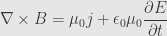
The other two of Maxwell’s equations come automatically from taking the potentials as fundamental and coming up with the electric and magnetic fields from them.