The Higgs Mechanism part 3: Gauge Symmetries
This is part three of a four-part discussion of the idea behind how the Higgs field does its thing. Read Part 1 and Part 2 first.
Now we’re starting to get to the really meaty stuff. We talked about the phase symmetry of the complex scalar field:
which basically wants to express the idea that the physics of this field only really depends on the length of the complex field values 
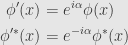
To answer this, we “gauge” the symmetry and make it local. The origin of the term is fascinating, but takes us too far afield. The upshot is that we now have the symmetry transformation:

where 

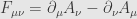
And here’s the big problem: since
and similarly for 
and makes the whole Lagrangian symmetric.
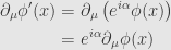
On the other hand, what do we see now?
![\displaystyle\begin{aligned}\partial_\mu\phi'(x)&=\partial_\mu\left(e^{i\alpha(x)}\phi(x)\right)\\&=e^{i\alpha(x)}\partial_\mu\phi(x)+i\partial_\mu\alpha(x)e^{i\alpha(x)}\phi(x)\\&=e^{i\alpha(x)}\left[\partial_\mu\phi(x)+i\partial_\mu\alpha(x)\phi(x)\right]\end{aligned}](https://s0.wp.com/latex.php?latex=%5Cdisplaystyle%5Cbegin%7Baligned%7D%5Cpartial_%5Cmu%5Cphi%27%28x%29%26%3D%5Cpartial_%5Cmu%5Cleft%28e%5E%7Bi%5Calpha%28x%29%7D%5Cphi%28x%29%5Cright%29%5C%5C%26%3De%5E%7Bi%5Calpha%28x%29%7D%5Cpartial_%5Cmu%5Cphi%28x%29%2Bi%5Cpartial_%5Cmu%5Calpha%28x%29e%5E%7Bi%5Calpha%28x%29%7D%5Cphi%28x%29%5C%5C%26%3De%5E%7Bi%5Calpha%28x%29%7D%5Cleft%5B%5Cpartial_%5Cmu%5Cphi%28x%29%2Bi%5Cpartial_%5Cmu%5Calpha%28x%29%5Cphi%28x%29%5Cright%5D%5Cend%7Baligned%7D&bg=e6e6e6&fg=333333&s=0&c=20201002)
We pick up this extra term when we differentiate, and it ruins the symmetry.
The way out is to add another field that can “soak up” this extra term. Since the derivative is a vector, we introduce a vector field 
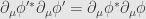
Next, we introduce a new derivative operator: 

And we calculate
![\displaystyle\begin{aligned}D_\mu\phi'(x)&=\partial_\mu\left(e^{i\alpha(x)}\phi(x)\right)-ieA_\mu'(x)e^{i\alpha(x)}\phi(x)\\&=e^{i\alpha(x)}\partial_\mu\phi(x)+i\partial_\mu\alpha(x)e^{i\alpha(x)}\phi(x)-ieA_\mu(x)e^{i\alpha(x)}\phi(x)-i\partial_\mu\alpha(x)e^{i\alpha(x)}\phi(x)\\&=e^{i\alpha(x)}\left[\partial_\mu\phi(x)-ieA_\mu(x)\phi(x)\right]\\&=e^{i\alpha(x)}D_\mu\phi(x)\end{aligned}](https://s0.wp.com/latex.php?latex=%5Cdisplaystyle%5Cbegin%7Baligned%7DD_%5Cmu%5Cphi%27%28x%29%26%3D%5Cpartial_%5Cmu%5Cleft%28e%5E%7Bi%5Calpha%28x%29%7D%5Cphi%28x%29%5Cright%29-ieA_%5Cmu%27%28x%29e%5E%7Bi%5Calpha%28x%29%7D%5Cphi%28x%29%5C%5C%26%3De%5E%7Bi%5Calpha%28x%29%7D%5Cpartial_%5Cmu%5Cphi%28x%29%2Bi%5Cpartial_%5Cmu%5Calpha%28x%29e%5E%7Bi%5Calpha%28x%29%7D%5Cphi%28x%29-ieA_%5Cmu%28x%29e%5E%7Bi%5Calpha%28x%29%7D%5Cphi%28x%29-i%5Cpartial_%5Cmu%5Calpha%28x%29e%5E%7Bi%5Calpha%28x%29%7D%5Cphi%28x%29%5C%5C%26%3De%5E%7Bi%5Calpha%28x%29%7D%5Cleft%5B%5Cpartial_%5Cmu%5Cphi%28x%29-ieA_%5Cmu%28x%29%5Cphi%28x%29%5Cright%5D%5C%5C%26%3De%5E%7Bi%5Calpha%28x%29%7DD_%5Cmu%5Cphi%28x%29%5Cend%7Baligned%7D&bg=e6e6e6&fg=333333&s=0&c=20201002)
So the derivative 

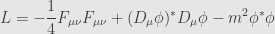
which is now symmetric under the gauged symmetry transformations.
It may not be apparent, but this Lagrangian does contain interaction terms. We can expand out the second term to find:

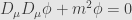
Our rules of thumb tell us that if we vary the Lagrangian with respect to

which — if we expand out 

The charge-current, in particular, we can write as

or, in a gauge-invariant manner, as
![\displaystyle j_\mu=-i\left[\phi^*D_\mu\phi-(D_\mu\phi)^*\phi\right]](https://s0.wp.com/latex.php?latex=%5Cdisplaystyle+j_%5Cmu%3D-i%5Cleft%5B%5Cphi%5E%2AD_%5Cmu%5Cphi-%28D_%5Cmu%5Cphi%29%5E%2A%5Cphi%5Cright%5D&bg=e6e6e6&fg=333333&s=0&c=20201002)
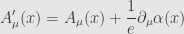
which is just the conserved current from last time with the regular derivatives replaced by covariant ones. Similarly, varying with respect to the field 
and, when this holds, we can show that 
So we’ve found that if we take the global symmetry of the complex scalar field and “gauge” it, something like electromagnetism naturally pops out, and the particle of the complex scalar field interacts with it like charged particles interact with the real electromagnetic field.
9 Comments »
RSS Feeds


That derivative operator is reminiscent of canonical momentum. Are they related?
When quantizing, the derivative with respect to a coordinate is indeed related to the “momentum operator” conjugate to that coordinate. I’m sticking to classical field theory here, though.
What does this “covariant derivative” have to do with the covariant derivative as usually defined on a bundle with a connection over a manifold? As far as I can tell, you’re still working in Lorentzian space-time.
That is an excellent question, Greg. I’ll start answering it by saying we’re actually working over Lorentzian spacetime, in that our fields are the sections of some fiber bundle over this space, and in this case the gauge group is . The
. The  fields are actually the components — analogous to the Christoffel symbols — of a connection on the associated principal fiber bundle.
Incidentally, that’s why there’s the in the covariant derivative formula:
  is really a
  -valued field.
[…] discussion of the idea behind how the Higgs field does its thing. Read Part 1, Part 2, and Part 3 […]
Pingback by The Higgs Mechanism part 4: Symmetry Breaking « The Unapologetic Mathematician | July 19, 2012 |
[…] “The Higgs Mechanism part 2: Examples of Lagrangian Field Equations,” July 17, “The Higgs Mechanism part 3: Gauge Symmetries,” July 18, y “The Higgs Mechanism part 4: Symmetry Breaking,” July 19. […]
Pingback by Las matemáticas del bosón de Higgs, para las abuelas cansadas de cháchara (Parte I) « Francis (th)E mule Science's News | July 19, 2012 |
[…] The Higgs Mechanism part 3: Gauge Symmetries […]
Pingback by The Unapologetic Mathematician Tackles the Higgs Mechanism | Whiskey…Tango…Foxtrot? | July 20, 2012 |
[…] “The Higgs Mechanism part 2: Examples of Lagrangian Field Equations,” July 17, “The Higgs Mechanism part 3: Gauge Symmetries,” July 18, y “The Higgs Mechanism part 4: Symmetry Breaking,” July 19. Recomiendo […]
Pingback by Las matemáticas del bosón de Higgs, para las abuelas cansadas de cháchara (Parte I) | Bosón de Higgs | La Ciencia de la Mula Francis | November 1, 2017 |