Let’s say that we have a one-dimensional distribution on a manifold  . Around any point
  we can find a patch
  and an everywhere-nonzero vector field
  on so that
  spans
spans  for every
  . Then we know we can find a chart
  around
  such that
  on
on  . Then the curve with coordinates
  and
and  for all other
  is a one-dimensional integral submanifold of
  through .
Now, this doesn’t always work for every distribution . It turns out that the key ingredient is that all one-dimensional distributions are integrable; we can show that any integrable  -dimensional distribution has an integrable submanifold through any point .
To give an even more detailed statement, let be a -dimensional integrable distribution on . for every there is a chart with  ,
,  , and so that for any
  the set
  is an integral submanifold of . Further, any connected integral submanifold of comes in this way.
Since this statement is purely local we can get away with working in some set of local coordinates to start with, although obviously not the one we’re trying to find. As such, we will assume that  , that
  , and that
  is spanned by the
  for
for  . We’ll also let
  be the projection onto the first components, so
  is an isomorphism. By parallel translation,
  for all
  in a neighborhood of
  .
.
Now, like we did yesterday we can use these isomorphisms to build vector fields  on belonging to that are
  -related to the
  on
on  . Then
 ![\pi_*[X_i,X_j]=[D_i,D_j]=0](https://s0.wp.com/latex.php?latex=%5Cpi_%2A%5BX_i%2CX_j%5D%3D%5BD_i%2CD_j%5D%3D0&bg=e6e6e6&fg=333333&s=0&c=20201002) , but since is integrable we know that
, but since is integrable we know that ![[X_i,X_j]\in\Delta](https://s0.wp.com/latex.php?latex=%5BX_i%2CX_j%5D%5Cin%5CDelta&bg=e6e6e6&fg=333333&s=0&c=20201002) . Since
. Since  is an isomorphism on , we conclude that
 ![[X_1,X_j]=0](https://s0.wp.com/latex.php?latex=%5BX_1%2CX_j%5D%3D0&bg=e6e6e6&fg=333333&s=0&c=20201002) . Now we can find a coordinate patch around with
. Now we can find a coordinate patch around with  on , just as in the one-dimensional case. It’s no loss of generality to tweak it until we have . This gives us an integral submanifold through the origin.
But our assertion goes further! Let  , where
  is the complementary projection to . This map has maximal rank everywhere, so we know that for each
  the preimage
  is an
is an  -dimensional submanifold
  . The tangent space to
  consists of exactly those vectors in the kernel of
  , but since
  is a diffeomorphism these are exactly those vectors
  such that
  is in the kernel of
  — those
  .
.
Conversely, if is a connected integral manifold of contained in . If  , then
  is in , which is spanned by the
  for . Thus
  . And so
  for all
  . Since is connected,
  is constant, and thus comes from picking a value
  for each
  .
.
June 30, 2011
Posted by John Armstrong |
Differential Topology, Topology |
Leave a comment
Given a -dimensional distribution on an  -dimensional manifold , we say that a -dimensional submanifold
  is an “integral submanifold” of if
  for every
  . That is, if the subspace of
  spanned by the images of vectors from
  is exactly
  .
.
This is a lot like an integral curve, with one slight distinction: in the case on an integral curve we also demand that the length of  match that of
  , not just the direction (up to sign).
Now, if for every there exists an integral submanifold  of with
  , then is integrable. Indeed, let and
  belong to . Since
  is an isomorphism of vector spaces at every point, we can find
  and
and  that are
  -related to and , respectively. That is,
  for all , and similarly for and . But then we know that
 ![[X,Y]_{\iota(q)}=\iota_*[\tilde{X},\tilde{Y}]_q](https://s0.wp.com/latex.php?latex=%5BX%2CY%5D_%7B%5Ciota%28q%29%7D%3D%5Ciota_%2A%5B%5Ctilde%7BX%7D%2C%5Ctilde%7BY%7D%5D_q&bg=e6e6e6&fg=333333&s=0&c=20201002) , and so
, and so ![[X,Y]_{\iota(q)}\in\iota_*\mathcal{T}_qN=\Delta_{\iota(q)}](https://s0.wp.com/latex.php?latex=%5BX%2CY%5D_%7B%5Ciota%28q%29%7D%5Cin%5Ciota_%2A%5Cmathcal%7BT%7D_qN%3D%5CDelta_%7B%5Ciota%28q%29%7D&bg=e6e6e6&fg=333333&s=0&c=20201002) .
.
June 30, 2011
Posted by John Armstrong |
Differential Topology, Topology |
2 Comments
A vector field defines a one-dimensional subspace of  at any point with
  : the subspace spanned by
  . If is everywhere nonzero, then it defines a one-dimensional subspace of each tangent space. A distribution generalizes this sort of thing to higher dimensions.
To this end, we define a -dimensional distribution on an -dimensional manifold to be a map  , where is a -dimensional subspace of . Further, we require that this map be “smooth”, in the sense that for any
  there exists some neighborhood of and vector fields
  such that the vectors
  span
span  for each
  .
.
Notice here that the  don’t have to work for the whole manifold . Indeed, we will see that in many cases there are no everywhere-nonzero vector fields on a manifold . But over a small patch we might more easily find vector fields that are linearly independent at each point, and thus define a smooth -dimensional distribution over . Then more general smooth distributions come from patching these sorts of smooth distributions together.
A vector field on “belongs to” a distribution — which we write  — if
— if  for all . We say that is “integrable” if
 ![[X,Y]\in\Delta](https://s0.wp.com/latex.php?latex=%5BX%2CY%5D%5Cin%5CDelta&bg=e6e6e6&fg=333333&s=0&c=20201002) for all and belonging to .
for all and belonging to .
Every one-dimensional manifold is integrable. To see this, we note that if and belong to then  for some constant
  , at least at those points where
  . Thus we see that
![\displaystyle[X,Y]=[fY,Y]=f[Y,Y]-(Yf)Y=-(Yf)Y](https://s0.wp.com/latex.php?latex=%5Cdisplaystyle%5BX%2CY%5D%3D%5BfY%2CY%5D%3Df%5BY%2CY%5D-%28Yf%29Y%3D-%28Yf%29Y&bg=e6e6e6&fg=333333&s=0&c=20201002)
and so ![[X,Y]](https://s0.wp.com/latex.php?latex=%5BX%2CY%5D&bg=e6e6e6&fg=333333&s=0&c=20201002) is proportional to , and thus belongs to . To handle points where
is proportional to , and thus belongs to . To handle points where  , we can put the scalar multiplier on the other side.
June 28, 2011
Posted by John Armstrong |
Differential Topology, Topology |
7 Comments
Today we’ll prove the assertions we made last time: if and are vector fields with flows  and
and  , respectively in some neighborhood of some point , we define the curve
](https://s0.wp.com/latex.php?latex=%5Cdisplaystyle+c%28t%29%3D%5Cleft%5B%5CPhi_%7B-t%7D%5Ccirc%5CPhi_%7B-t%7D%5Ccirc%5CPsi_t%5Ccirc%5CPhi_t%5Cright%5D%28p%29&bg=e6e6e6&fg=333333&s=0&c=20201002)
We assert that for any smooth  we have
![\displaystyle\begin{aligned}(f\circ c)'(0)&=0\\\frac{1}{2}(f\circ c)''(0)&=[X,Y]_p(f)\end{aligned}](https://s0.wp.com/latex.php?latex=%5Cdisplaystyle%5Cbegin%7Baligned%7D%28f%5Ccirc+c%29%27%280%29%26%3D0%5C%5C%5Cfrac%7B1%7D%7B2%7D%28f%5Ccirc+c%29%27%27%280%29%26%3D%5BX%2CY%5D_p%28f%29%5Cend%7Baligned%7D&bg=e6e6e6&fg=333333&s=0&c=20201002)
To show the first, we define the three “rectangles”
\\V_2(s,t)&=\left[\Phi_{-s}\circ\Psi_t\circ\Phi_t\right](p)\\V_3(s,t)&=\left[\Psi_{-s}\circ\Phi_{-t}\circ\Psi_t\circ\Phi_t\right](p)\end{aligned}](https://s0.wp.com/latex.php?latex=%5Cdisplaystyle%5Cbegin%7Baligned%7DV_1%28s%2Ct%29%26%3D%5Cleft%5B%5CPsi_s%5Ccirc%5CPhi_t%5Cright%5D%28p%29%5C%5CV_2%28s%2Ct%29%26%3D%5Cleft%5B%5CPhi_%7B-s%7D%5Ccirc%5CPsi_t%5Ccirc%5CPhi_t%5Cright%5D%28p%29%5C%5CV_3%28s%2Ct%29%26%3D%5Cleft%5B%5CPsi_%7B-s%7D%5Ccirc%5CPhi_%7B-t%7D%5Ccirc%5CPsi_t%5Ccirc%5CPhi_t%5Cright%5D%28p%29%5Cend%7Baligned%7D&bg=e6e6e6&fg=333333&s=0&c=20201002)
Notice that  ,
,  , and
, and  . The chain rule lets us then calculate:

as asserted. As for the other assertion, we start by observing

Using the fact that  we can turn the first term on the right into

Now, similar tedious calculations that make the big one above look like idle doodling give us two more identities:
![\displaystyle\begin{aligned}\frac{\partial^2(f\circ V_3)}{\partial s\partial t}(0,0)&=-Y_pYf\\\frac{\partial^2(f\circ V_3)}{\partial t^2}(0,0)&=Y_pYf+2[X,Y]_pf\end{aligned}](https://s0.wp.com/latex.php?latex=%5Cdisplaystyle%5Cbegin%7Baligned%7D%5Cfrac%7B%5Cpartial%5E2%28f%5Ccirc+V_3%29%7D%7B%5Cpartial+s%5Cpartial+t%7D%280%2C0%29%26%3D-Y_pYf%5C%5C%5Cfrac%7B%5Cpartial%5E2%28f%5Ccirc+V_3%29%7D%7B%5Cpartial+t%5E2%7D%280%2C0%29%26%3DY_pYf%2B2%5BX%2CY%5D_pf%5Cend%7Baligned%7D&bg=e6e6e6&fg=333333&s=0&c=20201002)
and we conclude that
![\displaystyle(f\circ c)''(0)=2[X,Y]_pf](https://s0.wp.com/latex.php?latex=%5Cdisplaystyle%28f%5Ccirc+c%29%27%27%280%29%3D2%5BX%2CY%5D_pf&bg=e6e6e6&fg=333333&s=0&c=20201002)
as asserted.
June 27, 2011
Posted by John Armstrong |
Differential Topology, Topology |
Leave a comment
We again pick up the question we posed earlier about what the bracket measures. Clearly it should have something to do with flows and their failure to commute. So we consider vector fields and with flows and , respectively.
Now, starting with a point and given some small time displacement  we can flow along and then —
 ](https://s0.wp.com/latex.php?latex=%5Cleft%5B%5CPsi_t%5Ccirc%5CPhi_t%5Cright%5D%28p%29&bg=e6e6e6&fg=333333&s=0&c=20201002) — or we can flow along and then —
— or we can flow along and then — ](https://s0.wp.com/latex.php?latex=%5Cleft%5B%5CPhi_t%5Ccirc%5CPsi_t%5Cright%5D%28p%29&bg=e6e6e6&fg=333333&s=0&c=20201002) — and get two (potentially different) points in . Unfortunately, we can’t just take their difference as we could when measuring the failure of algebra elements to commute.
— and get two (potentially different) points in . Unfortunately, we can’t just take their difference as we could when measuring the failure of algebra elements to commute.
However, we do have something rather closely related: the commutator in the sense of a group. That is, we can flow forwards along , then along , then backwards along and then backwards along to get the point  :
:
](https://s0.wp.com/latex.php?latex=%5Cdisplaystyle+c%28t%29%3D%5Cleft%5B%5CPsi_%7B-t%7D%5Ccirc%5CPhi_%7B-t%7D%5Ccirc%5CPsi_t%5Ccirc%5CPhi_t%5Cright%5D%28p%29&bg=e6e6e6&fg=333333&s=0&c=20201002)
If  and
and  were to commute this would just be the constant curve
  , but in general it’s a smooth curve passing through at
  . The bracket
 ![[X,Y]_p](https://s0.wp.com/latex.php?latex=%5BX%2CY%5D_p&bg=e6e6e6&fg=333333&s=0&c=20201002) will indicate the direction in which passes through , and something about its speed.
will indicate the direction in which passes through , and something about its speed.
Now, it turns out that the derivative always vanishes at . In fact, is more closely related to the “second derivative” of  , though it’s not immediately clear what this means. Indeed, we can define for any in an interval around , but
  , and there is in general no good way to compare these vectors for different values of .
Instead, we will prove the following two facts for any smooth — here “smoothness” entails twice differentiability — where is any neighborhood of :
The first indicates that  . Indeed, if
  then we could surely find some
  which changes in the direction it points, which would give a nonzero value to
  . The second gives the result we’re really after, as Taylor’s theorem applied to
  shows us that
![\displaystyle[X,Y]_p(f)=\frac{1}{2}(f\circ c)''(0)=\lim\limits_{t\to0}\frac{\left[f\circ c\right](t)-\left[f\circ c\right](0)}{t^2}](https://s0.wp.com/latex.php?latex=%5Cdisplaystyle%5BX%2CY%5D_p%28f%29%3D%5Cfrac%7B1%7D%7B2%7D%28f%5Ccirc+c%29%27%27%280%29%3D%5Clim%5Climits_%7Bt%5Cto0%7D%5Cfrac%7B%5Cleft%5Bf%5Ccirc+c%5Cright%5D%28t%29-%5Cleft%5Bf%5Ccirc+c%5Cright%5D%280%29%7D%7Bt%5E2%7D&bg=e6e6e6&fg=333333&s=0&c=20201002)
And thus the bracket indeed is the second (and lowest) order term in describing the direction of as it passes through .
June 23, 2011
Posted by John Armstrong |
Differential Topology, Topology |
1 Comment
Sorry for the delay; I’ve been swamped at my actual job the last couple days.
Anyway, I left off last time by pointing out that coordinate vector fields commute:
![\displaystyle\left[\frac{\partial}{\partial x^i},\frac{\partial}{\partial x^j}\right]=0](https://s0.wp.com/latex.php?latex=%5Cdisplaystyle%5Cleft%5B%5Cfrac%7B%5Cpartial%7D%7B%5Cpartial+x%5Ei%7D%2C%5Cfrac%7B%5Cpartial%7D%7B%5Cpartial+x%5Ej%7D%5Cright%5D%3D0&bg=e6e6e6&fg=333333&s=0&c=20201002)
Today I want to show a certain converse: if we have vector fields on some open region  that are linearly independent at some
  and which commute —
 ![[X_i,X_j]=0](https://s0.wp.com/latex.php?latex=%5BX_i%2CX_j%5D%3D0&bg=e6e6e6&fg=333333&s=0&c=20201002) for all
for all  and
and  — then we can find some coordinate chart around so that the are the first coordinate vector fields. That is,

In particular, if is a vector field with  then there is a coordinate chart around with
  .
.
If is any chart, then we can describe the th coordinate vector field by saying it’s the unique vector field on that is -related to the th partial derivative in  . That is, we’re trying to prove that:
  on
on  .
.
In fact, we can further simplify our claim by assuming that , , and  — that the vector fields agree at the point
  . Indeed, if
  is any coordinate map taking to then we can define the vector fields
  on . These must have vanishing brackets because we can calculate:
![\displaystyle\begin{aligned}{}[Y_i,Y_j]&=[z_*\circ X_i\circ z^{-1},z_*\circ X_j\circ z^{-1}]\\&=z_*\circ[X_i,X_j]\circ z^{-1}\\&=z_*\circ0\circ z^{-1}=0\end{aligned}](https://s0.wp.com/latex.php?latex=%5Cdisplaystyle%5Cbegin%7Baligned%7D%7B%7D%5BY_i%2CY_j%5D%26%3D%5Bz_%2A%5Ccirc+X_i%5Ccirc+z%5E%7B-1%7D%2Cz_%2A%5Ccirc+X_j%5Ccirc+z%5E%7B-1%7D%5D%5C%5C%26%3Dz_%2A%5Ccirc%5BX_i%2CX_j%5D%5Ccirc+z%5E%7B-1%7D%5C%5C%26%3Dz_%2A%5Ccirc0%5Ccirc+z%5E%7B-1%7D%3D0%5Cend%7Baligned%7D&bg=e6e6e6&fg=333333&s=0&c=20201002)
What’s more, if  is a local diffeomorphism of with
  , then
  is a coordinate map satisfying our assertion.
Now, let  be the flow of , and let
  be a small enough neighborhood of that we can define
  by
by
](https://s0.wp.com/latex.php?latex=%5Cdisplaystyle+f%28a_1%2C%5Cdots%2Ca_n%29%3D%5Cleft%5B%5CPhi%5E1_%7Ba_1%7D%5Ccirc%5Cdots%5Ccirc%5CPhi%5Ek_%7Ba_k%7D%5Cright%5D%280%2C%5Cdots%2C0%2Ca_%7Bk%2B1%7D%2C%5Cdots%2Ca_n%29&bg=e6e6e6&fg=333333&s=0&c=20201002)
The order that the flows come in here doesn’t matter, since we’re assuming that the — and thus their flows — commute. Anyway, given any smooth test function  on we can check
-\left[\phi\circ f\right](a_1,a_2,\dots,a_n)\right]\\&=\lim\limits_{h\to0}\frac{1}{h}\left[\left[\phi\circ\Phi^1_{a_1+h}\circ\dots\circ\Phi^k_{a_k}\right](0,\dots,0,a_{k+1},\dots,a_n)-\left[\phi\circ f\right](a)\right]\\&=\lim\limits_{h\to0}\frac{1}{h}\left[\left[\phi\circ\Phi_h\circ\Phi^1_{a_1}\circ\dots\circ\Phi^k_{a_k}\right](0,\dots,0,a_{k+1},\dots,a_n)-\left[\phi\circ f\right](a)\right]\\&=\lim\limits_{h\to0}\frac{1}{h}\left[\left[\phi\circ\Phi_h\right](a)-\left[\phi\circ f\right](a)\right]\\&=\left(X_1\right)_{f(a)}(\phi)\end{aligned}](https://s0.wp.com/latex.php?latex=%5Cdisplaystyle%5Cbegin%7Baligned%7D%5Cleft%28f_%2AD_1%5Cright%29_a%5Cphi%26%3D%5Cleft%28D_1%5Cright%29_a%28%5Cphi%5Ccirc+f%29%5C%5C%26%3D%5Clim%5Climits_%7Bh%5Cto0%7D%5Cfrac%7B1%7D%7Bh%7D%5Cleft%5B%5Cleft%5B%5Cphi%5Ccirc+f%5Cright%5D%28a_1%2Bh%2Ca_2%2C%5Cdots%2Ca_n%29-%5Cleft%5B%5Cphi%5Ccirc+f%5Cright%5D%28a_1%2Ca_2%2C%5Cdots%2Ca_n%29%5Cright%5D%5C%5C%26%3D%5Clim%5Climits_%7Bh%5Cto0%7D%5Cfrac%7B1%7D%7Bh%7D%5Cleft%5B%5Cleft%5B%5Cphi%5Ccirc%5CPhi%5E1_%7Ba_1%2Bh%7D%5Ccirc%5Cdots%5Ccirc%5CPhi%5Ek_%7Ba_k%7D%5Cright%5D%280%2C%5Cdots%2C0%2Ca_%7Bk%2B1%7D%2C%5Cdots%2Ca_n%29-%5Cleft%5B%5Cphi%5Ccirc+f%5Cright%5D%28a%29%5Cright%5D%5C%5C%26%3D%5Clim%5Climits_%7Bh%5Cto0%7D%5Cfrac%7B1%7D%7Bh%7D%5Cleft%5B%5Cleft%5B%5Cphi%5Ccirc%5CPhi_h%5Ccirc%5CPhi%5E1_%7Ba_1%7D%5Ccirc%5Cdots%5Ccirc%5CPhi%5Ek_%7Ba_k%7D%5Cright%5D%280%2C%5Cdots%2C0%2Ca_%7Bk%2B1%7D%2C%5Cdots%2Ca_n%29-%5Cleft%5B%5Cphi%5Ccirc+f%5Cright%5D%28a%29%5Cright%5D%5C%5C%26%3D%5Clim%5Climits_%7Bh%5Cto0%7D%5Cfrac%7B1%7D%7Bh%7D%5Cleft%5B%5Cleft%5B%5Cphi%5Ccirc%5CPhi_h%5Cright%5D%28a%29-%5Cleft%5B%5Cphi%5Ccirc+f%5Cright%5D%28a%29%5Cright%5D%5C%5C%26%3D%5Cleft%28X_1%5Cright%29_%7Bf%28a%29%7D%28%5Cphi%29%5Cend%7Baligned%7D&bg=e6e6e6&fg=333333&s=0&c=20201002)
That is,  . To see this for any other , simply swap around the flows to bring to the front.
We can also check that
-\left[\phi\circ f\right](0,\dots,0)\right]\\&=\lim\limits_{h\to0}\frac{1}{h}\left[\phi(0,\dots,0,h,0,\dots,0)-\phi(0,\dots,0)\right]\\&=\left(D_{k+i}\right)_0\phi\end{aligned}](https://s0.wp.com/latex.php?latex=%5Cdisplaystyle%5Cbegin%7Baligned%7D%5Cleft%28f_%2AD_%7Bk%2Bi%7D%5Cright%29_0%5Cphi%26%3D%5Cleft%28D_%7Bk%2Bi%7D%5Cright%29_0%28%5Cphi%5Ccirc+f%29%5C%5C%26%3D%5Clim%5Climits_%7Bh%5Cto0%7D%5Cfrac%7B1%7D%7Bh%7D%5Cleft%5B%5Cleft%5B%5Cphi%5Ccirc+f%5Cright%5D%280%2C%5Cdots%2C0%2Ch%2C0%2C%5Cdots%2C0%29-%5Cleft%5B%5Cphi%5Ccirc+f%5Cright%5D%280%2C%5Cdots%2C0%29%5Cright%5D%5C%5C%26%3D%5Clim%5Climits_%7Bh%5Cto0%7D%5Cfrac%7B1%7D%7Bh%7D%5Cleft%5B%5Cphi%280%2C%5Cdots%2C0%2Ch%2C0%2C%5Cdots%2C0%29-%5Cphi%280%2C%5Cdots%2C0%29%5Cright%5D%5C%5C%26%3D%5Cleft%28D_%7Bk%2Bi%7D%5Cright%29_0%5Cphi%5Cend%7Baligned%7D&bg=e6e6e6&fg=333333&s=0&c=20201002)
Thus  is the identity transformation on
  . The inverse function theorem now tells us that there is a chart around with
  , which will then satisfy our assertions.
June 22, 2011
Posted by John Armstrong |
Differential Topology, Topology |
1 Comment
Now, what does the Lie bracket of two vector fields really measure? We’ve gone through all this time defining and manipulating a bunch of algebraic expressions, but this is supposed to be geometry! What does the bracket actually mean? It turns out that the bracket of two vector fields measures the extent to which their flows fail to commute.
We won’t work this all out today, but we’ll start with an important first step: the bracket of two vector fields vanishes if and only if their flows commute. That is, if and are vector fields with flows  and , respectively, then
 ![[X,Y]=0](https://s0.wp.com/latex.php?latex=%5BX%2CY%5D%3D0&bg=e6e6e6&fg=333333&s=0&c=20201002) if and only if
if and only if  for all
  and .
and .
First we assume that the flows commute. As we just saw last time, the fact that for all means that is -invariant. That is,  . But this implies that the Lie derivative
  vanishes, and we know that
 ![L_XY=[X,Y]](https://s0.wp.com/latex.php?latex=L_XY%3D%5BX%2CY%5D&bg=e6e6e6&fg=333333&s=0&c=20201002) .
.
Conversely, let’s assume that . For any we can define the curve  in the tangent space by
  . Since the Lie derivative vanishes, we know that
  , and I say that
  for all , or (equivalently) that
  .
.
Fixing any we can set  . Then we calculate
![\displaystyle\begin{aligned}c_p'(s)&=\lim\limits_{\Delta s\to0}\frac{c_p(s+\Delta s)-c_p(s)}{\Delta s}\\&=\lim\limits_{\Delta s\to0}\frac{1}{\Delta s}\left[\Phi_{-(s+\Delta s)*}\circ Y\circ\Phi_{s+\Delta s}(p)-\Phi_{-s*}\circ Y\circ\Phi_s(p)\right]\\&=\lim\limits_{\Delta s\to0}\frac{1}{\Delta s}\Phi_{-s*}\left[\left[\Phi_{-\Delta s*}\circ Y\circ\Phi_{\Delta s}\right]\left(\Phi_s(p)\right)-Y\left(\Phi_s(p)\right)\right]\\&=\Phi_{-s*}\lim\limits_{\Delta s\to0}\frac{1}{\Delta s}\left[\left[\Phi_{-\Delta s*}\circ Y\circ\Phi_{\Delta s}\right](q)-Y(q)\right]\\&=\Phi_{-s*}c_q'(0)=\Phi_{-s*}0=0\end{aligned}](https://s0.wp.com/latex.php?latex=%5Cdisplaystyle%5Cbegin%7Baligned%7Dc_p%27%28s%29%26%3D%5Clim%5Climits_%7B%5CDelta+s%5Cto0%7D%5Cfrac%7Bc_p%28s%2B%5CDelta+s%29-c_p%28s%29%7D%7B%5CDelta+s%7D%5C%5C%26%3D%5Clim%5Climits_%7B%5CDelta+s%5Cto0%7D%5Cfrac%7B1%7D%7B%5CDelta+s%7D%5Cleft%5B%5CPhi_%7B-%28s%2B%5CDelta+s%29%2A%7D%5Ccirc+Y%5Ccirc%5CPhi_%7Bs%2B%5CDelta+s%7D%28p%29-%5CPhi_%7B-s%2A%7D%5Ccirc+Y%5Ccirc%5CPhi_s%28p%29%5Cright%5D%5C%5C%26%3D%5Clim%5Climits_%7B%5CDelta+s%5Cto0%7D%5Cfrac%7B1%7D%7B%5CDelta+s%7D%5CPhi_%7B-s%2A%7D%5Cleft%5B%5Cleft%5B%5CPhi_%7B-%5CDelta+s%2A%7D%5Ccirc+Y%5Ccirc%5CPhi_%7B%5CDelta+s%7D%5Cright%5D%5Cleft%28%5CPhi_s%28p%29%5Cright%29-Y%5Cleft%28%5CPhi_s%28p%29%5Cright%29%5Cright%5D%5C%5C%26%3D%5CPhi_%7B-s%2A%7D%5Clim%5Climits_%7B%5CDelta+s%5Cto0%7D%5Cfrac%7B1%7D%7B%5CDelta+s%7D%5Cleft%5B%5Cleft%5B%5CPhi_%7B-%5CDelta+s%2A%7D%5Ccirc+Y%5Ccirc%5CPhi_%7B%5CDelta+s%7D%5Cright%5D%28q%29-Y%28q%29%5Cright%5D%5C%5C%26%3D%5CPhi_%7B-s%2A%7Dc_q%27%280%29%3D%5CPhi_%7B-s%2A%7D0%3D0%5Cend%7Baligned%7D&bg=e6e6e6&fg=333333&s=0&c=20201002)
Now this means that is -invariant for all , meaning that and commute for all and , as asserted.
As a special case, if is a coordinate patch then we have the coordinate vector fields . The fact that partial derivatives commute means that the brackets disappear:
This corresponds to the fact that adding to the th coordinate and to the th coordinate can be done in either order. That is, their flows commute.
June 18, 2011
Posted by John Armstrong |
Differential Topology, Topology |
3 Comments
It’s all well and good to define the Lie derivative, but it’s not exactly straightforward to calculate it from the definition. For one thing, it requires knowing the flow of the vector field , which requires solving a differential equation that might be difficult in practice. Luckily, there’s an easier way.
But first, a lemma: if  is an interval containing
  ,
,  is an open set, and
  is a differentiable function with
  for all
  , then there is another differentiable function
  such that

This is basically just like a lemma we proved for functions on star-shaped neighborhoods. Indeed, it suffices to set
Now let ,  , and
, and  is the local flow of a vector field on a region containing . Consider the function
  , which satisfies the condition of the above lemma. We can thus write
-f(q)=tg(t,q)](https://s0.wp.com/latex.php?latex=%5Cdisplaystyle%5Cleft%5Bf%5Ccirc%5CPhi_t%5Cright%5D%28q%29-f%28q%29%3Dtg%28t%2Cq%29&bg=e6e6e6&fg=333333&s=0&c=20201002)
for some . Or if we write  we can write

We also can see that  . And so we can write
-t\left[(Yg_{-t})\circ\Phi_t\right](p)\end{aligned}](https://s0.wp.com/latex.php?latex=%5Cdisplaystyle%5Cbegin%7Baligned%7D%5CPhi_%7B-t%2A%7DY_%7B%5CPhi_t%28p%29%7D%28f%29%26%3DY_%7B%5CPhi_t%28p%29%7D%5Cleft%28f%5Ccirc%5CPhi_%7B-t%7D%5Cright%29%5C%5C%26%3DY_%7B%5CPhi_t%28p%29%7D%5Cleft%28f-tg_%7B-t%7D%5Cright%29%5C%5C%26%3D%5Cleft%5B%28Yf%29%5Ccirc%5CPhi_t%5Cright%5D%28p%29-t%5Cleft%5B%28Yg_%7B-t%7D%29%5Ccirc%5CPhi_t%5Cright%5D%28p%29%5Cend%7Baligned%7D&bg=e6e6e6&fg=333333&s=0&c=20201002)
So now we calculate
-t\left[(Yg_{-t})\circ\Phi_t\right](p)-Yf(p)}{t}\\&=\lim\limits_{t\to0}\frac{\left[(Yf)\circ\Phi_t\right](p)-Yf(p)}{t}-\lim\limits_{t\to0}\left[(Yg_{-t})\circ\Phi_t\right](p)\end{aligned}](https://s0.wp.com/latex.php?latex=%5Cdisplaystyle%5Cbegin%7Baligned%7D%28L_XY%29_pf%26%3D%5Clim%5Climits_%7Bt%5Cto0%7D%5Cfrac%7B%5CPhi_%7B-t%2A%7DY_%7B%5CPhi_%7Bt%7D%28p%29%7D%28f%29-Y_pf%7D%7Bt%7D%5C%5C%26%3D%5Clim%5Climits_%7Bt%5Cto0%7D%5Cfrac%7B%5Cleft%5B%28Yf%29%5Ccirc%5CPhi_t%5Cright%5D%28p%29-t%5Cleft%5B%28Yg_%7B-t%7D%29%5Ccirc%5CPhi_t%5Cright%5D%28p%29-Yf%28p%29%7D%7Bt%7D%5C%5C%26%3D%5Clim%5Climits_%7Bt%5Cto0%7D%5Cfrac%7B%5Cleft%5B%28Yf%29%5Ccirc%5CPhi_t%5Cright%5D%28p%29-Yf%28p%29%7D%7Bt%7D-%5Clim%5Climits_%7Bt%5Cto0%7D%5Cleft%5B%28Yg_%7B-t%7D%29%5Ccirc%5CPhi_t%5Cright%5D%28p%29%5Cend%7Baligned%7D&bg=e6e6e6&fg=333333&s=0&c=20201002)
Last time we wrote the action of on a smooth function as
-\phi(p)}{t}](https://s0.wp.com/latex.php?latex=%5Cdisplaystyle+X_p%28%5Cphi%29%3D%5Clim%5Climits_%7Bt%5Cto0%7D%5Cfrac%7B%5Cleft%5B%5Cphi%5Ccirc%5CPhi_t%5Cright%5D%28p%29-%5Cphi%28p%29%7D%7Bt%7D&bg=e6e6e6&fg=333333&s=0&c=20201002)
which pattern we can recognize in our formula. We thus continue
-Yf(p)}{t}-\lim\limits_{t\to0}\left[(Yg_{-t})\circ\Phi_t\right](p)\\&=X_pYf-Yg_0(p)\\&=X_pYf-Y_pXf\\&=[X,Y]_pf\end{aligned}](https://s0.wp.com/latex.php?latex=%5Cdisplaystyle%5Cbegin%7Baligned%7D%28L_XY%29_pf%26%3D%5Clim%5Climits_%7Bt%5Cto0%7D%5Cfrac%7B%5Cleft%5B%28Yf%29%5Ccirc%5CPhi_t%5Cright%5D%28p%29-Yf%28p%29%7D%7Bt%7D-%5Clim%5Climits_%7Bt%5Cto0%7D%5Cleft%5B%28Yg_%7B-t%7D%29%5Ccirc%5CPhi_t%5Cright%5D%28p%29%5C%5C%26%3DX_pYf-Yg_0%28p%29%5C%5C%26%3DX_pYf-Y_pXf%5C%5C%26%3D%5BX%2CY%5D_pf%5Cend%7Baligned%7D&bg=e6e6e6&fg=333333&s=0&c=20201002)
That is, for any two vector fields the Lie derivative is actually the same as the bracket .
June 16, 2011
Posted by John Armstrong |
Differential Topology, Topology |
1 Comment
Let’s go back to the way a vector field on a manifold gives us a “derivative” of smooth functions  . If
. If  is a smooth vector field it has a maximal flow which gives a one-parameter family of diffeomorphisms, which we can think of as “moving forward along by .
Now given a smooth function we use this as if we were taking a derivative from all the way back in single-variable calculus: measure at , flow forward by  and measure at
  , take the difference, divide by , and take the limit as approaches zero:
![\displaystyle\begin{aligned}\lim\limits_{\Delta t\to0}\frac{f\left(\Phi_{\Delta t}(p)\right)-f(p)}{\Delta t}&=\lim\limits_{\Delta t\to0}\frac{f\left(\Phi(\Delta t,p)\right)-f\left(\Phi(0,p)\right)}{\Delta t}\\&=\frac{\partial}{\partial t}f\left(\Phi(\Delta t,p)\right)\Big\vert_{t=0}\\&=\left[df(p)\right]\left(\Phi_*\left(\frac{\partial}{\partial t}(t,p)\Big\vert_{t=0}\right)\right)\\&=\left[df(p)\right]\left(X(\Phi(0,p))\right)\\&=\left[df(p)\right]\left(X(p)\right)\\&=Xf(p)\end{aligned}](https://s0.wp.com/latex.php?latex=%5Cdisplaystyle%5Cbegin%7Baligned%7D%5Clim%5Climits_%7B%5CDelta+t%5Cto0%7D%5Cfrac%7Bf%5Cleft%28%5CPhi_%7B%5CDelta+t%7D%28p%29%5Cright%29-f%28p%29%7D%7B%5CDelta+t%7D%26%3D%5Clim%5Climits_%7B%5CDelta+t%5Cto0%7D%5Cfrac%7Bf%5Cleft%28%5CPhi%28%5CDelta+t%2Cp%29%5Cright%29-f%5Cleft%28%5CPhi%280%2Cp%29%5Cright%29%7D%7B%5CDelta+t%7D%5C%5C%26%3D%5Cfrac%7B%5Cpartial%7D%7B%5Cpartial+t%7Df%5Cleft%28%5CPhi%28%5CDelta+t%2Cp%29%5Cright%29%5CBig%5Cvert_%7Bt%3D0%7D%5C%5C%26%3D%5Cleft%5Bdf%28p%29%5Cright%5D%5Cleft%28%5CPhi_%2A%5Cleft%28%5Cfrac%7B%5Cpartial%7D%7B%5Cpartial+t%7D%28t%2Cp%29%5CBig%5Cvert_%7Bt%3D0%7D%5Cright%29%5Cright%29%5C%5C%26%3D%5Cleft%5Bdf%28p%29%5Cright%5D%5Cleft%28X%28%5CPhi%280%2Cp%29%29%5Cright%29%5C%5C%26%3D%5Cleft%5Bdf%28p%29%5Cright%5D%5Cleft%28X%28p%29%5Cright%29%5C%5C%26%3DXf%28p%29%5Cend%7Baligned%7D&bg=e6e6e6&fg=333333&s=0&c=20201002)
Note that even if is not complete we do always have some interval around on which is defined and this difference quotient makes sense.
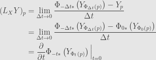
So far this is just a complicated (but descriptive!) way of restating something we already knew about. But now we can take this same approach and apply it to other vector fields. So if  is another smooth vector field, we define the “Lie derivative” of by as:

Again we evaluate at both and , but here’s where a trick comes in: we can’t compare these two vectors directly, since they live at different points on , and thus in different tangent spaces. So in order to compensate we use the flow itself to move backwards from back to , and use the derivative  to carry along the vector
  .
.
We can come up with an alternate version of this formula by using similar techniques to those above:
That is, if we define the curve  in the tangent space then
  . This would seem to make it live in the tangent space to
  — that is, in
  — but remember that since is a vector space we identify it with all of its tangent spaces. Thus
  , just like
  is.
is.
June 15, 2011
Posted by John Armstrong |
Differential Topology, Topology |
5 Comments


\right)\right)\\&=\left[f\circ\Phi\circ\left(1_\mathbb{R}\times f^{-1}\right)\right](t,p)\end{aligned}](https://s0.wp.com/latex.php?latex=%5Cdisplaystyle%5Cbegin%7Baligned%7D%5Ctilde%7B%5CPhi%7D%28t%2Cp%29%26%3Df%5Cleft%28%5CPhi_t%5Cleft%28f%5E%7B-1%7D%28p%29%5Cright%29%5Cright%29%5C%5C%26%3Df%5Cleft%28%5CPhi%5Cleft%28t%2Cf%5E%7B-1%7D%28p%29%5Cright%29%5Cright%29%5C%5C%26%3Df%5Cleft%28%5CPhi%5Cleft%28%5Cleft%5B1_%5Cmathbb%7BR%7D%5Ctimes+f%5E%7B-1%7D%5Cright%5D%28t%2Cp%29%5Cright%29%5Cright%29%5C%5C%26%3D%5Cleft%5Bf%5Ccirc%5CPhi%5Ccirc%5Cleft%281_%5Cmathbb%7BR%7D%5Ctimes+f%5E%7B-1%7D%5Cright%29%5Cright%5D%28t%2Cp%29%5Cend%7Baligned%7D&bg=e6e6e6&fg=333333&s=0&c=20201002)
![\displaystyle\begin{aligned}\tilde{\Phi}_*\left(\frac{\partial}{\partial t}(t,p)\right)&=f_*\left(\Phi_*\left((1_\mathbb{R}\times f^{-1})_*\left(\iota_{p*}\left(\frac{d}{dt}(t)\right)\right)\right)\right)\\&=f_*\left(\Phi_*\left(\left((1_\mathbb{R}\times f^{-1})\circ\iota_p\right)_*\left(\frac{d}{dt}(t)\right)\right)\right)\\&=f_*\left(\Phi_*\left(\iota_{f^{-1}(p)*}\left(\frac{d}{dt}(t)\right)\right)\right)\\&=f_*\left(X\left(\Phi\left(t,f^{-1}(p)\right)\right)\right)\\&=\left[f_*\circ X\circ\Phi\right]\left(t,f^{-1}(p)\right)\\&=\left[f_*\circ X\circ f^{-1}\circ f\circ\Phi\circ(1_\mathbb{R}\times f^{-1})\right](t,p)\\&=\left[\tilde{X}\circ\tilde{\Phi}\right](t,p)\\&=\tilde{X}\left(\tilde{\Phi}(t,p)\right)\end{aligned}](https://s0.wp.com/latex.php?latex=%5Cdisplaystyle%5Cbegin%7Baligned%7D%5Ctilde%7B%5CPhi%7D_%2A%5Cleft%28%5Cfrac%7B%5Cpartial%7D%7B%5Cpartial+t%7D%28t%2Cp%29%5Cright%29%26%3Df_%2A%5Cleft%28%5CPhi_%2A%5Cleft%28%281_%5Cmathbb%7BR%7D%5Ctimes+f%5E%7B-1%7D%29_%2A%5Cleft%28%5Ciota_%7Bp%2A%7D%5Cleft%28%5Cfrac%7Bd%7D%7Bdt%7D%28t%29%5Cright%29%5Cright%29%5Cright%29%5Cright%29%5C%5C%26%3Df_%2A%5Cleft%28%5CPhi_%2A%5Cleft%28%5Cleft%28%281_%5Cmathbb%7BR%7D%5Ctimes+f%5E%7B-1%7D%29%5Ccirc%5Ciota_p%5Cright%29_%2A%5Cleft%28%5Cfrac%7Bd%7D%7Bdt%7D%28t%29%5Cright%29%5Cright%29%5Cright%29%5C%5C%26%3Df_%2A%5Cleft%28%5CPhi_%2A%5Cleft%28%5Ciota_%7Bf%5E%7B-1%7D%28p%29%2A%7D%5Cleft%28%5Cfrac%7Bd%7D%7Bdt%7D%28t%29%5Cright%29%5Cright%29%5Cright%29%5C%5C%26%3Df_%2A%5Cleft%28X%5Cleft%28%5CPhi%5Cleft%28t%2Cf%5E%7B-1%7D%28p%29%5Cright%29%5Cright%29%5Cright%29%5C%5C%26%3D%5Cleft%5Bf_%2A%5Ccirc+X%5Ccirc%5CPhi%5Cright%5D%5Cleft%28t%2Cf%5E%7B-1%7D%28p%29%5Cright%29%5C%5C%26%3D%5Cleft%5Bf_%2A%5Ccirc+X%5Ccirc+f%5E%7B-1%7D%5Ccirc+f%5Ccirc%5CPhi%5Ccirc%281_%5Cmathbb%7BR%7D%5Ctimes+f%5E%7B-1%7D%29%5Cright%5D%28t%2Cp%29%5C%5C%26%3D%5Cleft%5B%5Ctilde%7BX%7D%5Ccirc%5Ctilde%7B%5CPhi%7D%5Cright%5D%28t%2Cp%29%5C%5C%26%3D%5Ctilde%7BX%7D%5Cleft%28%5Ctilde%7B%5CPhi%7D%28t%2Cp%29%5Cright%29%5Cend%7Baligned%7D&bg=e6e6e6&fg=333333&s=0&c=20201002)

