The Higgs Mechanism part 2: Examples of Lagrangian Field Equations

This is part two of a four-part discussion of the idea behind how the Higgs field does its thing. Read Part 1 first.

Okay, now that we’re sold on the Lagrangian formalism you can rest easy: I’m not going to go through the gory details of any more variational calculus. I do want to clear a couple notational things out of the way, though. They might not all matter for the purposes of our discussion, but better safe than sorry.

First off, I’m going to use a coordinate system where the speed of light is 1. That is, if my unit of time is seconds, my unit of distance is light-seconds. Mostly this helps keep annoying constants out of the way of the equations; physicists do this basically all the time. The other thing is that I’m going to work in four-dimensional spacetime, meaning we’ve got four coordinates: $x_0$ , $x_1$ , $x_2$ , and $x_3$ . We calculate dot products by writing $v\cdot w=v_1w_1+v_2w_2+v_3w_3-v_0w_0$ . Yes, that minus sign is weird, but that’s just how spacetime works.

Also instead of writing spacetime vectors, I’m going to write down their components, indexed by a subscript that’s meant to run from 0 to 3. Usually this will be a Greek letter from the middle of the alphabet like $\mu$ or $\nu$ . Similarly, instead of writing $\nabla$ for the vector composed of the four spacetime derivatives of a field I’ll just write down the derivatives, and I’ll write $\partial_\mu f$ instead of $\frac{\partial f}{\partial x_\mu}$ .

Along with writing down components instead of vectors I won’t be writing dot products explicitly. Instead I’ll use the common convention that when the same index appears twice we’re supposed to sum over it, remembering that the zero component gets a minus sign. That is, $v_\mu w_\mu$ is the dot product from above. Similarly, we can multiply a matrix with entries $A_{\mu\nu}$ by a vector $v_\nu$ to get $w_\mu=A_{\mu\nu}v_\nu$ ; notice how the summed index $\nu$ gets “eaten up” in the process.

Okay, now even without going through the details there’s a fair bit we can infer from general rules of thumb. Any term in the Lagrangian that contains a derivative of the field we’re varying is almost always going to be the squared-length of that derivative, and the resulting term in the variational equations will be the negative of a second derivative of the field. For any term that involves the plain field we basically take its derivative as if the field were a variable. Any term that doesn’t involve the field at all just goes away. And since we prefer positive second-derivative terms to negative ones, we usually flip the sign of the resulting equation; since the other side is zero this doesn’t matter.

So if, for instance, we have the following Lagrangian of a complex scalar field $\phi$ :

$\displaystyle L=\partial_\mu\phi^*\partial_\mu\phi-m^2\phi^*\phi$

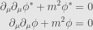
we get two equations by varying the field $\phi$ and its complex conjugate $\phi^*$ separately:

$\displaystyle\begin{aligned}\partial_\mu\partial_\mu\phi^*+m^2\phi^*&=0\\\partial_\mu\partial_\mu\phi+m^2\phi&=0\end{aligned}$

It may not seem to make sense to vary the field and its complex conjugate separately, but the two equations we get at the end are basically the same anyway, so we’ll let this slide for now. Anyway, what we get is a second derivative of $\phi$ set equal to $m^2$ times $\phi$ itself, which we call the “Klein-Gordon wave equation” for $\phi$ . Since the term $m^2\phi^*\phi$ gives rise to the term $m^2\phi$ in the field equations, we call this the “mass term”.

In the case of electromagnetism in a vacuum we just have the electromagnetic fields and no charge or current distribution. We use the Faraday field 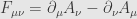$F_{\mu\nu}=\partial_\mu A_\nu-\partial_\nu A_\mu$ to write down the Lagrangian

$\displaystyle L=-\frac{1}{4}F_{\mu\nu}F_{\mu\nu}$

which gives rise to the field equations

$\displaystyle\partial_\mu F_{\mu\nu}=0$

or, equivalently in terms of the potential field $A$ :

$\displaystyle\begin{aligned}\partial_\mu\partial_\mu A_\nu&=0\\\partial_\nu A_\nu&=0\end{aligned}$

The second equation just expresses a choice we can make to always consider divergence-free potentials without affecting the predictions of electromagnetism; the first equation looks like the Klein-Gordon equation again, except there’s no mass term. Indeed, we know that photons — the particles associated to the electromagnetic field — have no rest mass!

Turning back to the complex scalar field, we notice that there’s a certain symmetry to this Lagrangian. Specifically, if we replace $\phi(x)$ and $\phi^*$ by

$\displaystyle\begin{aligned}\phi'(x)&=e^{i\alpha}\phi(x)\\\phi'^*(x)&=e^{-i\alpha}\phi^*(x)\end{aligned}$

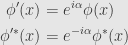
for any constant $\alpha$ , we get the same result. This is important, and it turns out to be a clue that leads us — I won’t go into the details — to consider the quantity

$\displaystyle j_\mu=-i(\phi^*\partial_\mu\phi-\phi\partial_\mu\phi^*)$

This is interesting because we can calculate

$\displaystyle\begin{aligned}\partial_\mu j_\mu&=-i\partial_\mu(\phi^*\partial_\mu\phi-\phi\partial_\mu\phi^*)\\&=-i(\partial_\mu\phi^*\partial_\mu\phi+\phi^*\partial_\mu\partial_\mu\phi-\partial_\mu\phi\partial_\mu\phi^*-\phi\partial_\mu\partial_\mu\phi^*)\\&=-i(\phi^*\partial_\mu\partial_\mu\phi-\phi\partial_\mu\partial_\mu\phi^*)\\&=-i(-m^2\phi^*\phi+m^2\phi\phi^*)\\&=0\end{aligned}$

where we’ve used the results of the Klein-Gordon equations. Since $\partial_\mu j_\mu=0$ , this is a suitable vector field to use as a charge-current distribution; the equation just says that charge is conserved! That is, we can write down a Lagrangian involving both electromagnetism — that is, our “massless vector field” $A_\mu$ and our scalar field:

$\displaystyle L=-\frac{1}{4}F_{\mu\nu}F_{\mu\nu}-ej_\mu A_\mu$

where $e$ is a “coupling constant” that tells us how important the “interaction term” involving both $j_\mu$ and $A_\mu$ is. If it’s zero, then the fields don’t actually interact at all, but if it’s large then they affect each other very strongly.

July 17, 2012 - Posted by John Armstrong | Higgs Mechanism, Mathematical Physics, Special Topics

9 Comments »

This is a bit disorienting to try to read when you don’t follow the standard convention of matching upper and lower indexes. Also confusing when you say that \partial_\mu is used for \partial/\partial x_\mu whereas it’s normally got the other sign (\partial/\partial x^\mu).

Note also that there’s a missing equality in the equation just after “which gives rise to the field equations”.

Comment by peeterjoot | July 17, 2012 | Reply
Well, physicists themselves often disregard the idea of covariant-vs.-contravariant indices, especially when the metric is standard; I didn’t feel like going into all that mess of an explanation here.

As for the typo, thanks; fixed.

Comment by John Armstrong | July 18, 2012 | Reply
Question to physicists: Is it really that hard to put a big capital sigma to the left of your equation and put all of the summed indices below it separated by commas?

I realise who are we to quibble with Einstein over notation, but it’s pretty frustrating.

Comment by Pseudonym | July 18, 2012 | Reply
You’d have to do it on a term-by-term basis, since indices in different terms have little to do with each other.

Comment by John Armstrong | July 18, 2012 | Reply
[…] of a four-part discussion of the idea behind how the Higgs field does its thing. Read Part 1 and Part 2 […]

Pingback by The Higgs Mechanism part 3: Gauge Symmetries « The Unapologetic Mathematician | July 18, 2012 | Reply
[…] four of a four-part discussion of the idea behind how the Higgs field does its thing. Read Part 1, Part 2, and Part 3 […]

Pingback by The Higgs Mechanism part 4: Symmetry Breaking « The Unapologetic Mathematician | July 19, 2012 | Reply
[…] Mathematician en “The Higgs Mechanism part 1: Lagrangians,” July 16, “The Higgs Mechanism part 2: Examples of Lagrangian Field Equations,” July 17, “The Higgs Mechanism part 3: Gauge Symmetries,” July 18, y “The […]

Pingback by Las matemáticas del bosón de Higgs, para las abuelas cansadas de cháchara (Parte I) « Francis (th)E mule Science's News | July 19, 2012 | Reply
[…] The Higgs Mechanism part 2: Examples of Lagrangian Field Equations […]

Pingback by The Unapologetic Mathematician Tackles the Higgs Mechanism | Whiskey…Tango…Foxtrot? | July 20, 2012 | Reply
[…] Mathematician en “The Higgs Mechanism part 1: Lagrangians,” July 16, “The Higgs Mechanism part 2: Examples of Lagrangian Field Equations,” July 17, “The Higgs Mechanism part 3: Gauge Symmetries,” July 18, y “The […]

Pingback by Las matemáticas del bosón de Higgs, para las abuelas cansadas de cháchara (Parte I) | Bosón de Higgs | La Ciencia de la Mula Francis | November 1, 2017 | Reply

About this weblog

This is mainly an expository blath, with occasional high-level excursions, humorous observations, rants, and musings. The main-line exposition should be accessible to the “Generally Interested Lay Audience”, as long as you trace the links back towards the basics. Check the sidebar for specific topics (under “Categories”).

I’m in the process of tweaking some aspects of the site to make it easier to refer back to older topics, so try to make the best of it for now.

RSS Feeds

RSS - Posts
RSS - Comments
Feedback

Got something to say? Anonymous questions, comments, and suggestions at Formspring.me!
Subjects

Subjects
Archives

July 2012

M T W T F S S

1

2 3 4 5 6 7 8

9 10 11 12 13 14 15

16 17 18 19 20 21 22

23 24 25 26 27 28 29

30 31

« Mar Aug »
Search for:

The Unapologetic Mathematician

Mathematics for the interested outsider