Okay, back to linear algebra and inner product spaces. I want to look at the matrix of a linear map between finite-dimensional inner product spaces.
So, let’s say  and
and  are inner product spaces with orthonormal bases
  and
and  , respectively, and let
  be a linear map from one to the other. We know that we can write down the matrix
  for
for  , where the matrix entries are defined as the coefficients in the expansion

But now that we’ve got an inner product on , it will be easy to extract these coefficients. Just consider the inner product
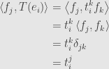
Presto! We have a nice, neat function that takes a linear map and gives us back the  –
– entry in its matrix — with respect to the appropriate bases, naturally.
But this is also the root of a subtle, but important, shift in understanding what a matrix entry actually is. Up until now, we’ve thought of matrix entries as artifacts which happen to be useful for calculations. But now we’re very explicitly looking at the question “what scalar shows up in this slot of the matrix of a linear map with respect to these particular bases?” as a function. In fact,  is now not just some scalar value peculiar to the transformation at hand; it’s now a particular linear functional on the space of all transformations
  .
.
And, really, what do the indices and matter? If we rearranged the bases we’d find the same function in a new place in the new array. We could have taken this perspective before, with any vector space, but what we couldn’t have asked before is this more general question: “Given a vector  and a vector
  , how much does the image
  is made up of
  ?” This new question only asks about these two particular vectors, and doesn’t care anything about any of the other basis vectors that may (or may not!) be floating around. But in the context of an inner product space, this question has an answer:

Any function of this form we’ll call a “matrix element”. We can use such matrix elements to probe linear transformations even without full bases to work with, sort of like the way we generalized “elements” of an abelian group to “members” of an object in an abelian category. This is especially useful when we move to the infinite-dimensional context and might find it hard to come up with a proper basis to make a matrix with. Instead, we can work with the collection of all matrix elements and use it in arguments in place of some particular collection of matrix elements which happen to come from particular bases.
Now it would be really neat if matrix elements themselves formed a vector space, but the situation’s sort of like when we constructed tensor products. Matrix elements are like the “pure” tensors  . They (far more than) span the space
  of all linear functionals on the space of linear transformations, just like pure tensors span the whole tensor product space. But almost all linear functionals have to be written as a nontrivial sum of matrix elements — they usually can’t be written with just one. Still, since they span we know that many properties which hold for all matrix elements will immediately hold for all linear functionals on .
May 29, 2009
Posted by John Armstrong |
Algebra, Linear Algebra |
2 Comments
Forgot to hit “publish” earlier…
So we’ve seen that the unit complex numbers can be written in the form  where
where  denotes the (signed) angle between the point on the circle and
  . We’ve also seen that this view behaves particularly nicely with respect to multiplication: multiplying two unit complex numbers just adds their angles. Today I want to extend this viewpoint to the whole complex plane.
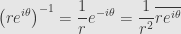
If we start with any nonzero complex number  , we can find its absolute value
  . This is a positive real number which we’ll also call
  . We can factor this out of
  to find
  . The complex number in parentheses has unit absolute value, and so we can write it as for some between
  and
and  . Thus we’ve written our complex number in the form

where the positive real number is the absolute value of , and — a real number in the range ![\left(-\pi,\pi\right]](https://s0.wp.com/latex.php?latex=%5Cleft%28-%5Cpi%2C%5Cpi%5Cright%5D&bg=e6e6e6&fg=333333&s=0&c=20201002) — is the angle makes with the reference point . But this is exactly how we define the polar coordinates
— is the angle makes with the reference point . But this is exactly how we define the polar coordinates  back in high school math courses.
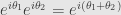
Just like we saw for unit complex numbers, this notation is very well behaved with respect to multiplication. Given complex numbers  and
and  we calculate their product:

That is, we multiply their lengths (as we already knew) and add their angles, just like before. This viewpoint also makes division simple:

In particular we see that
so multiplicative inverses are given in terms of complex conjugates and magnitudes as we already knew.
Powers (including roots) are also easy, which gives rise to easy ways to remember all those messy double- and triple-angle formulæ from trigonometry:


Other angle addition formulæ should be similarly easy to verify from this point.
In general, since we consider complex numbers multiplicatively so often it will be convenient to have this polar representation of complex numbers at hand. It will also generalize nicely, as we will see.
May 29, 2009
Posted by John Armstrong |
Fundamentals, Numbers |
3 Comments
Yesterday we saw that the unit-length complex numbers are all of the form , where measures the oriented angle from around to the point in question. Since the absolute value of a complex number is multiplicative, we know that the product of two unit-length complex numbers is again of unit length. We can also see this using the exponential property:
So multiplying two unit-length complex numbers corresponds to adding their angles.
That is, the complex numbers on the unit circle form a group under multiplication of complex numbers — a subgroup of the multiplicative group of the complex field — and we even have an algebraic description of this group. The function sending the real number to the point on the circle is a homomorphism from the additive group of real numbers to the circle group. Since every point on the circle has such a representative, it’s an epimorphism. What is the kernel? It’s the collection of real numbers satisfying

that is, must be an integral multiple of  — an element of the subgroup
  . So, algebraically, the circle group is the quotient
  . Or, isomorphically, we can just write
  .
.
Something important has happened here. We have in hand two distinct descriptions of the circle. One we get by putting the unit-length condition on points in the plane. The other we get by taking the real line and “wrapping” it around itself periodically. I haven’t really mentioned the topologies, but the first approach inherits the subspace topology from the topology on the complex numbers, while the second approach inherits the quotient topology from the topology on the real numbers. And it turns out that the identity map from one version of the circle to the other one is actually a homeomorphism, which further shows that the two descriptions give us “the same” result.
What’s really different between the two cases is how they generalize. I’ll probably come back to these in more detail later, but for now I’ll point out that the first approach generalizes to spheres in higher dimensions, while the second generalizes to higher-dimensional tori. Thus the circle is sometimes called the one-dimensional sphere  , and sometimes called the one-dimensional torus
  , and each one calls to mind a slightly different vision of the same basic object of study.
May 27, 2009
Posted by John Armstrong |
Algebra, Fundamentals, Group theory, Numbers |
3 Comments
When I first talked about complex numbers there was one perspective I put off, and now need to come back to. It makes deep use of Euler’s formula, which ties exponentials and trigonometric functions together in the relation

where we’ve written  for
for  and used the exponential property.
Remember that we have a natural basis for the complex numbers as a vector space over the reals:  . If we ask that this natural basis be orthonormal, we get a real inner product on complex numbers, which in turn gives us lengths and angles. In fact, this notion of length is exactly that which we used to define the absolute value of a complex number, in order to get a topology on the field.
So what happens when we look at ? First, we can calculate its length using this inner product, getting

by the famous trigonometric identity. That is, every complex number of the form lies a unit distance from the complex number  .
.
In particular,  is a nice reference point among such points. We can use it as a fixed post in the complex plane, and measure the angle it makes with any other point. For example, we can calculate the inner product

and thus we find that the point makes an angle  with our fixed post
  , at least for
  . We see that traces a circle by increasing the angle in one direction as increases from to , and increasing the angle in the other direction as decreases from to . For values of outside this range, we can use the fact that

to see that the function is periodic with period . That is, we can add or subtract whatever multiple of we need to move within the range  . Thus, as varies the point traces out a circle of unit radius, going around and around with period , and every point on the unit circle has a unique representative of this form with in the given range.
May 26, 2009
Posted by John Armstrong |
Fundamentals, Numbers |
3 Comments
Many of the properties of the adjoint construction follow immediately from the contravariant functoriality of the duality we used in its construction. But they can also be determined from the adjoint relation

For example, if we have transformations  and , then the adjoint of their composite is the composite of their adjoints in the opposite order:
  . To check this, we write
,w\right\rangle_W&=\left\langle T\left(S(u)\right),w\right\rangle_W\\&=\left\langle S(u),T^*(w)\right\rangle_V\\&=\left\langle u,S^*\left(T^*(w)\right)\right\rangle_U\\&=\left\langle u,\left[S^*T^*\right](w)\right\rangle_W\end{aligned}](https://s0.wp.com/latex.php?latex=%5Cdisplaystyle%5Cbegin%7Baligned%7D%5Cleft%5Clangle%5Cleft%5BTS%5Cright%5D%28u%29%2Cw%5Cright%5Crangle_W%26%3D%5Cleft%5Clangle+T%5Cleft%28S%28u%29%5Cright%29%2Cw%5Cright%5Crangle_W%5C%5C%26%3D%5Cleft%5Clangle+S%28u%29%2CT%5E%2A%28w%29%5Cright%5Crangle_V%5C%5C%26%3D%5Cleft%5Clangle+u%2CS%5E%2A%5Cleft%28T%5E%2A%28w%29%5Cright%29%5Cright%5Crangle_U%5C%5C%26%3D%5Cleft%5Clangle+u%2C%5Cleft%5BS%5E%2AT%5E%2A%5Cright%5D%28w%29%5Cright%5Crangle_W%5Cend%7Baligned%7D&bg=e6e6e6&fg=333333&s=0&c=20201002)
It’s pretty straightforward to see that  . Then, since
  and
and  , we find that
  and
and  , which shows that
  .
.
Similarly, it’s easy to show that  . But the process isn’t quite linear. When we work over the complex numbers, we find that
  :
:
,w\right\rangle_W&=\left\langle T(\lambda v),w\right\rangle_W\\&=\left\langle\lambda v,T^*(w)\right\rangle_V\\&=\left\langle v,\bar{\lambda}T^*(w)\right\rangle_V\\&=\left\langle v,\left[\bar{\lambda}T^*\right](w)\right\rangle_V\end{aligned}](https://s0.wp.com/latex.php?latex=%5Cdisplaystyle%5Cbegin%7Baligned%7D%5Cleft%5Clangle%5Cleft%5B%5Clambda+T%5Cright%5D%28v%29%2Cw%5Cright%5Crangle_W%26%3D%5Cleft%5Clangle+T%28%5Clambda+v%29%2Cw%5Cright%5Crangle_W%5C%5C%26%3D%5Cleft%5Clangle%5Clambda+v%2CT%5E%2A%28w%29%5Cright%5Crangle_V%5C%5C%26%3D%5Cleft%5Clangle+v%2C%5Cbar%7B%5Clambda%7DT%5E%2A%28w%29%5Cright%5Crangle_V%5C%5C%26%3D%5Cleft%5Clangle+v%2C%5Cleft%5B%5Cbar%7B%5Clambda%7DT%5E%2A%5Cright%5D%28w%29%5Cright%5Crangle_V%5Cend%7Baligned%7D&bg=e6e6e6&fg=333333&s=0&c=20201002)
Now if we restrict our focus to endomorphisms of a single vector space , we see that the adjoint construction gives us an involutory (since  ), semilinear (since it applies the complex conjugate to scalar multiples) antiautomorphism of the algebra of endomorphisms of . That is, it’s like an automorphism, except it reverses the order of multiplication.
In a way, then, the adjoint behaves sort of like the complex conjugate itself does for the algebra of complex numbers (over the complex numbers we don’t notice the order of multiplication, but work with me here, people). This analogy goes pretty far, as we’ll see.
May 25, 2009
Posted by John Armstrong |
Algebra, Linear Algebra |
2 Comments
Since an inner product on a finite-dimensional vector space is a bilinear form, it provides two isomorphisms from to its dual  . And since an inner product is a symmetric bilinear form, these two isomorphisms are identical. But since duality is a (contravariant) functor, we have a dual transformation
  for every linear transformation . So what happens when we put these two together?
Say we start with linear transformation . We’ll build up a transformation from to which we’ll call the “adjoint” to . First we have the isomorphism  . Then we follow this with the dual transformation . Finally, we use the isomorphism
  . We’ll write
  for this composite, and rely on context to tell us whether we mean the dual or the adjoint (but because of the isomorphisms they’re secretly the same thing).
So why is this the adjoint? Let’s say we have vectors and . Then it turns out that
which should recall the relation between two adjoint functors. An important difference here is that there is no distinction between left- and right-adjoint transformations. The adjoint of an adjoint is the original transformation back again:  . This follows if we use the symmetry of the inner products on the relation above

Then since \right\rangle_W=0](https://s0.wp.com/latex.php?latex=%5Cleft%5Clangle+w%2C%5Cleft%5BT-T%5E%7B%2A%2A%7D%5Cright%5D%28v%29%5Cright%5Crangle_W%3D0&bg=e6e6e6&fg=333333&s=0&c=20201002) and the inner product on is nondegenerate, we must have
and the inner product on is nondegenerate, we must have  sending every
  to the zero vector in . Thus
  .
.
So let’s show this adjoint condition in the first place. On the left side, we have the result of applying the linear functional  to the vector
  . But this linear functional is simply the image of the vector under the isomorphism . So on the left, we’ve calculated the result of first applying to , and then applying this linear functional.
But the way we defined the dual transformation was such that we can instead apply the dual to the linear functional  , and then apply the resulting functional to , and we’ll get the same result. And the isomorphism tells us that there is some vector in
  so that the linear functional we’re now applying to is
  . That is, our value will be
  for some vector
  . Which one? The one we defined as
  .
.
I’ll admit that it sometimes takes a little getting used to the way adjoints and duals are the same, and also the subtleties of how they’re distinct. But it sinks in soon enough.
May 22, 2009
Posted by John Armstrong |
Algebra, Linear Algebra |
7 Comments
If all goes according to plan, a link to this post should show up on my Twitter feed shortly. Thanks to twitterfeed.
May 22, 2009
Posted by John Armstrong |
Uncategorized |
Leave a comment
I helped the Howard County and Baltimore County ARML teams practice tonight by joining the group of local citizens and team alumni to field a scrimmage team. As usual, my favorite part is the power question. It follows, as printed, but less the (unnecessary) diagrams:
Consider the function

which maps the real number  to the a coordinate in the
  –
– plane. Assume throughout that
  , ,
, ,  , , and
  are real numbers.
(1) Compute  ,
,  ,
,  ,
,  ,
,  , and
, and  . Sketch a plot of these points, superimposed on the unit circle.
(2) Show that  is one-to-one. That is, show that if
  , then
  .
.
(3) Let  be the intersection point between the unit circle and the line connecting
  and
and  . Prove that
  .
.
(4) Show that  is an ordered pair of rational numbers on the unit circle different from if and only if there is a rational number such that
  . (This result allows us to deduce that there are infinitely (countably) many rational points on the unit circle.)
According to problem 3,  is a particular geometric mapping of a single point on the real line to the unit circle. Now, we will be concerned with the relationship between the pairs of points, which will lead to a way of doing arithmetic by geometry. Use these definitions:
- Let
 be a “vertical pair” if either
  , or
, or  , or
, or  and
and  latex \phi(t)$ are two different points on the same vertical line.
- Let be a “horizontal pair” if either
 , or
, or  and are two different points on the same horizontal line.
- Let be a “diametric pair” if and are two different end points of the same diameter of the circle.
(5) (a) Prove that for all and , is a vertical pair if and only if  .
.
(b) Prove that for all and , is a horizontal pair if and only if  .
.
(c) Determine and prove a relationship between and that is a necessary and sufficient condition for to be a diametric pair.
(6) (a) Suppose that is not a vertical pair. Then, the straight line through them (if , use the tangent line to the circle at that point) intersects the -axis at the point  . Find
  in terms of and , and simplify and prove your answer.
(b) Draw the straight line through the point  and , where is the point described in problem (5a). Let
  denote the point of intersection of this line and the circle. Prove that
  .
.
(7) (a) Suppose that is not a horizontal pair. Then, the straight line through them (if , use the tangent line to the circle at that point) intersects the horizontal line  at the point
  . Find
  in terms of and , and simplify and prove your answer.
(b) Draw the straight line through the point  and , where is the point described in problem (6a). Let denote the point of intersection of this line and the circle. Prove that
  .
.
(8) Suppose , , , and are distinct real numbers such that  and such that the line containing
  and intersects the line containing
  and . Find the -coordinate of the intersection point in terms of and only.
(9) Let and be distinct real numbers such that  . Given only the unit circle, the – and – axes, the points and , and a straitedge (but no compass), determine a method to construct the point
  that uses no more than
  line segments. Prove why the construction works and provide a sketch.
(10) Given only the unit circle, the -and – axes, the point  , and a straightedge (but no compass), describe a method to construct the point
  .
.
May 21, 2009
Posted by John Armstrong |
Uncategorized |
2 Comments


