A Trace Criterion for Nilpotence

We’re going to need another way of identifying nilpotent endomorphisms. Let be two subspaces of endomorphisms on a finite-dimensional space , and let be the collection of such that sends into . If satisfies for all then is nilpotent.

The first thing we do is take the Jordan-Chevalley decomposition of — — and fix a basis that diagonalizes with eigenvalues . We define to be the -subspace of spanned by the eigenvalues. If we can prove that this space is trivial, then all the eigenvalues of must be zero, and thus itself must be zero.

We proceed by showing that any linear functional must be zero. Taking one, we define to be the endomorphism whose matrix with respect to our fixed basis is diagonal: . If is the corresponding basis of we can calculate that

Now we can find some polynomial such that ; there is no ambiguity here since if then the linearity of implies that

Further, picking we can see that , so has no constant term. It should be apparent that .

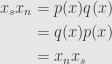
Now, we know that is the semisimple part of , so the Jordan-Chevalley decomposition lets us write it as a polynomial in with no constant term. But then we can write 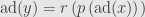. Since maps into , so does , and our hypothesis tells us that

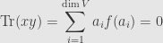
Hitting this with we find that the sum of the squares of the is also zero, but since these are rational numbers they must all be zero.

Thus, as we asserted, the only possible -linear functional on is zero, meaning that is trivial, all the eigenvalues of are zero, and is nipotent, as asserted.

Uses of the Jordan-Chevalley Decomposition

Now that we’ve given the proof, we want to mention a few uses of the Jordan-Chevalley decomposition.

First, we let be any finite-dimensional -algebra — associative, Lie, whatever — and remember that contains the Lie algebra of derivations . I say that if then so are its semisimple part and its nilpotent part ; it’s enough to show that is.

Just like we decomposed in the proof of the Jordan-Chevalley decomposition, we can break down into the eigenspaces of — or, equivalently, of . But this time we will index them by the eigenvalue: consists of those such that for sufficiently large .

Now we have the identity:

which is easily verified. If a sufficiently large power of applied to and a sufficiently large power of applied to are both zero, then for sufficiently large one or the other factor in each term will be zero, and so the entire sum is zero. Thus we verify that .

If we take and then , and thus . On the other hand,

And thus satisfies the derivation property

so and are both in .

For the other side we note that, just as the adjoint of a nilpotent endomorphism is nilpotent, the adjoint of a semisimple endomorphism is semisimple. Indeed, if is a basis of such that the matrix of is diagonal with eigenvalues , then we let be the standard basis element of , which is isomorphic to using the basis . It’s a straightforward calculation to verify that

and thus is diagonal with respect to this basis.

So now if is the Jordan-Chevalley decomposition of , then is semisimple and is nilpotent. They commute, since

Since is the decomposition of into a semisimple and a nilpotent part which commute with each other, it is the Jordan-Chevalley decomposition of .

The Jordan-Chevalley Decomposition (proof)

We now give the proof of the Jordan-Chevalley decomposition. We let have distinct eigenvalues with multiplicities , so the characteristic polynomial of is

We set so that is the direct sum of these subspaces, each of which is fixed by .

On the subspace , has the characteristic polynomial . What we want is a single polynomial such that

That is, has no constant term, and for each there is some such that

Thus, if we evaluate on the block we get .

To do this, we will make use of a result that usually comes up in number theory called the Chinese remainder theorem. Unfortunately, I didn’t have the foresight to cover number theory before Lie algebras, so I’ll just give the statement: any system of congruences — like the one above — where the moduli are relatively prime — as they are above, unless is an eigenvalue in which case just leave out the last congruence since we don’t need it — has a common solution, which is unique modulo the product of the separate moduli. For example, the system

has the solution , which is unique modulo . This is pretty straightforward to understand for integers, but it works as stated over any principal ideal domain — like — and, suitably generalized, over any commutative ring.

So anyway, such a exists, and it’s the we need to get the semisimple part of . Indeed, on any block differs from by stripping off any off-diagonal elements. Then we can just set and find . Any two polynomials in must commute — indeed we can simply calculate

Finally, if then so must any polynomial in , so the last assertion of the decomposition holds.

The only thing left is the uniqueness of the decomposition. Let’s say that is a different decomposition into a semisimple and a nilpotent part which commute with each other. Then we have , and all four of these endomorphisms commute with each other. But the left-hand side is semisimple — diagonalizable — but the right hand side is nilpotent, which means its only possible eigenvalue is zero. Thus and .

The Jordan-Chevalley Decomposition

We recall that any linear endomorphism of a finite-dimensional vector space over an algebraically closed field can be put into Jordan normal form: we can find a basis such that its matrix is the sum of blocks that look like

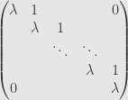
where is some eigenvalue of the transformation. We want a slightly more abstract version of this, and it hinges on the idea that matrices in Jordan normal form have an obvious diagonal part, and a bunch of entries just above the diagonal. This off-diagonal part is all in the upper-triangle, so it is nilpotent; the diagonalizable part we call “semisimple”. And what makes this particular decomposition special is that the two parts commute. Indeed, the block-diagonal form means we can carry out the multiplication block-by-block, and in each block one factor is a constant multiple of the identity, which clearly commutes with everything.

More generally, we will have the Jordan-Chevalley decomposition of an endomorphism: any can be written uniquely as the sum , where is semisimple — diagonalizable — and is nilpotent, and where and commute with each other.

Further, we will find that there are polynomials and — each of which with no constant term — such that and . And thus we will find that any endomorphism that commutes with with also commute with both and .

Finally, if is any pair of subspaces such that then the same is true of both and .

We will prove these next time, but let’s see that this is actually true of the Jordan normal form. The first part we’ve covered.

For the second, set aside the assertion about and ; any endomorphism commuting with either multiplies each block by a constant or shuffles similar blocks, and both of these operations commute with both and .

For the last part, we may as well assume that , since otherwise we can just restrict to . If then the Jordan normal form shows us that any complementary subspace to must be spanned by blocks with eigenvalue . In particular, it can only touch the last row of any such block. But none of these rows are in the range of either the diagonal or off-diagonal portions of the matrix.

Invariant Forms

A very useful structure to have on a complex vector space carrying a representation of a group is an “invariant form”. To start with, this is a complex inner product , which we recall means that it is

• linear in the second slot —
• conjugate symmetric —
• positive definite — for all

Again as usual these imply conjugate linearity in the first slot, so the form isn’t quite bilinear. Still, people are often sloppy and say “invariant bilinear form”.

Anyhow, now we add a new condition to the form. We demand that it be

• invariant under the action of —

Here I have started to write as shorthand for . We will only do this when the representation in question is clear from the context.

The inner product gives us a notion of length and angle. Invariance now tells us that these notions are unaffected by the action of . That is, the vectors and have the same length for all and . Similarly, the angle between vectors and is exactly the same as the angle between and . Another way to say this is that if the form is invariant for the representation , then the image of is actually contained in the orthogonal group [commenter Eric Finster, below, reminds me that since we’ve got a complex inner product we’re using the group of unitary transformations with respect to the inner product : ].

More important than any particular invariant form is this: if we have an invariant form on our space , then any reducible representation is decomposable. That is, if is a submodule, we can find another submodule so that as -modules.

If we just consider them as vector spaces, we already know this: the orthogonal complement is exactly the subspace we need, for . I say that if is a -invariant subspace of , then is as well, and so they are both submodules. Indeed, if , then we check that is as well:

where the first equality follows from the -invariance of our form; the second from the representation property; and the third from the fact that is an invariant subspace, so .

So in the presence of an invariant form, all finite-dimensional representations are “completely reducible”. That is, they can be decomposed as the direct sum of a number of irreducible submodules. If the representation is irreducible to begin with, we’re done. If not, it must have some submodule . Then the orthogonal complement is also a submodule, and we can write . Then we can treat both and the same way. The process must eventually bottom out, since each of and have dimension smaller than that of , which was finite to begin with. Each step brings the dimension down further and further, and it must stop by the time it reaches .

This tells us, for instance, that there can be no inner product on that is invariant under the representation of the group of integers we laid out at the end of last time. Indeed, that was an example of a reducible representation that is not decomposable, but if there were an invariant form it would have to decompose.

Topological Vector Spaces, Normed Vector Spaces, and Banach Spaces

Before we move on, we want to define some structures that blend algebraic and topological notions. These are all based on vector spaces. And, particularly, we care about infinite-dimensional vector spaces. Finite-dimensional vector spaces are actually pretty simple, topologically. For pretty much all purposes you have a topology on your base field , and the vector space (which is isomorphic to for some ) will get the product topology.

But for infinite-dimensional spaces the product topology is often not going to be particularly useful. For example, the space of functions is a product; we write to mean the product of one copy of for each point in . Limits in this topology are “pointwise” limits of functions, but this isn’t always the most useful way to think about limits of functions. The sequence

converges pointwise to a function for and . But we will find it useful to be able to ignore this behavior at the one isolated point and say that . It’s this connection with spaces of functions that brings such infinite-dimensional topological vector spaces into the realm of “functional analysis”.

Okay, so to get a topological vector space, we take a vector space and put a (surprise!) topology on it. But not just any topology will do: Remember that every point in a vector space looks pretty much like every other one. The transformation has an inverse , and it only makes sense that these be homeomorphisms. And to capture this, we put a uniform structure on our space. That is, we specify what the neighborhoods are of , and just translate them around to all the other points.

Now, a common way to come up with such a uniform structure is to define a norm on our vector space. That is, to define a function satisfying the three axioms

• For all vectors and scalars , we have .
• For all vectors and , we have .
• The norm is zero if and only if the vector is the zero vector.

Notice that we need to be working over a field in which we have a notion of absolute value, so we can measure the size of scalars. We might also want to do away with the last condition and use a “seminorm”. In any event, it’s important to note that though our earlier examples of norms all came from inner products we do not need an inner product to have a norm. In fact, there exist norms that come from no inner product at all.

So if we define a norm we get a “normed vector space”. This is a metric space, with a metric function defined by . This is nice because metric spaces are first-countable, and thus sequential. That is, we can define the topology of a (semi-)normed vector space by defining exactly what it means for a sequence of vectors to converge, and in particular what it means for them to converge to zero.

Finally, if we’ve got a normed vector space, it’s a natural question to ask whether or not this vector space is complete or not. That is, we have all the pieces in place to define Cauchy sequences in our vector space, and we would like for all of these sequences to converge under our uniform structure. If this happens — if we have a complete normed vector space — we call our structure a “Banach space”. Most of the spaces we’re concerned with in functional analysis are Banach spaces.

Again, for finite-dimensional vector spaces (at least over or ) this is all pretty easy; we can always define an inner product, and this gives us a norm. If our underlying topological field is complete, then the vector space will be as well. Even without considering a norm, convergence of sequences is just given component-by-component. But infinite-dimensional vector spaces get hairier. Since our algebraic operations only give us finite sums, we have to take some sorts of limits to even talk about most vectors in the space in the first place, and taking limits of such vectors could just complicate things further. Studying these interesting topologies and seeing how linear algebra — the study of vector spaces and linear transformations — behaves in the infinite-dimensional context is the taproot of functional analysis.

A Lemma on Reflections

Here’s a fact we’ll find useful soon enough as we talk about reflections. Hopefully it will also help get back into thinking about linear transformations and inner product spaces. However, if the linear algebra gets a little hairy (or if you’re just joining us) you can just take this fact as given. Remember that we’re looking at a real vector space equipped with an inner product .

Now, let’s say is some finite collection of vectors which span (it doesn’t matter if they’re linearly independent or not). Let be a linear transformation which leaves invariant. That is, if we pick any vector then the image will be another vector in . Let’s also assume that there is some -dimensional subspace which leaves completely untouched. That is, for every . Finally, say that there’s some so that (clearly ) and also that is invariant under . Then I say that and .

We’ll proceed by actually considering the transformation , and showing that this is the identity. First off, definitely fixes , since

so acts as the identity on the line . In fact, I assert that also acts as the identity on the quotient space . Indeed, acts trivially on , and every vector in has a unique representative in . And then acts trivially on , and every vector in has a unique representative in .

This does not, however, mean that acts trivially on any given complement of . All we really know at this point is that for every the difference between and is some scalar multiple of . On the other hand, remember how we found upper-triangular matrices before. This time we peeled off one vector and the remaining transformation was the identity on the remaining -dimensional space. This tells us that all of our eigenvalues are , and the characteristic polynomial is , where . We can evaluate this on the transformation to find that

Now let’s try to use the collection of vectors . We assumed that both and send vectors in back to other vectors in , and so the same must be true of . But there are only finitely many vectors (say of them) in to begin with, so must act as some sort of permutation of the vectors in . But every permutation in has an order that divides . That is, applying times must send every vector in back to itself. But since is a spanning set for , this means that , or that

So we have two polynomial relations satisfied by , and will clearly satisfy any linear combination of these relations. But Euclid’s algorithm shows us that we can write the greatest common divisor of these relations as a linear combination, and so must satisfy the greatest common divisor of and . It’s not hard to show that this greatest common divisor is , which means that we must have or .

It’s sort of convoluted, but there are some neat tricks along the way, and we’ll be able to put this result to good use soon.

Reflections

Before introducing my main question for the next series of posts, I’d like to talk a bit about reflections in a real vector space equipped with an inner product . If you want a specific example you can think of the space consisting of -tuples of real numbers . Remember that we’re writing our indices as superscripts, so we shouldn’t think of these as powers of some number , but as the components of a vector. For the inner product, you can think of the regular “dot product” .

Everybody with me? Good. Now that we’ve got our playing field down, we need to define a reflection. This will be an orthogonal transformation, which is just a fancy way of saying “preserves lengths and angles”. What makes it a reflection is that there’s some -dimensional “hyperplane” that acts like a mirror. Every vector in itself is just left where it is, and a vector on the line that points perpendicularly to will be sent to its negative — “reflecting” through the “mirror” of .

Any nonzero vector spans a line , and the orthogonal complement — all the vectors perpendicular to — forms an -dimensional subspace , which we can use to make just such a reflection. We’ll write for the reflection determined in this way by . We can easily write down a formula for this reflection:

It’s easy to check that if then , while if is perpendicular to — if — then , leaving the vector fixed. Thus this formula does satisfy the definition of a reflection through .

The amount that reflection moves in the above formula will come up a lot in the near future; enough so we’ll want to give it the notation . That is, we define:

Notice that this is only linear in , not in . You might also notice that this is exactly twice the length of the projection of the vector onto the vector . This notation isn’t standard, but the more common notation conflicts with other notational choices we’ve made on this weblog, so I’ve made an executive decision to try it this way.

Cramer’s Rule

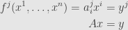
We’re trying to invert a function which is continuously differentiable on some region . That is we know that if is a point where , then there is a ball around where is one-to-one onto some neighborhood around . Then if is a point in , we’ve got a system of equations

that we want to solve for all the .

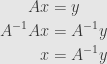
We know how to handle this if is defined by a linear transformation, represented by a matrix :

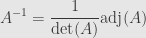
In this case, the Jacobian transformation is just the function itself, and so the Jacobian determinant is nonzero if and only if the matrix is invertible. And so our solution depends on finding the inverse and solving

This is the approach we’d like to generalize. But to do so, we need a more specific method of finding the inverse.

This is where Cramer’s rule comes in, and it starts by analyzing the way we calculate the determinant of a matrix . This formula

involves a sum over all the permutations , and we want to consider the order in which we add up these terms. If we fix an index , we can factor out each matrix entry in the th column:

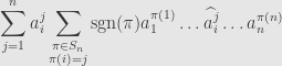
where the hat indicates that we omit the th term in the product. For a given value of , we can consider the restricted sum

which is times the determinant of the – “minor” of the matrix . That is, if we strike out the row and column of which contain and take the determinant of the remaining matrix, we multiply this by to get . These are the entries in the “adjugate” matrix .

What we’ve shown is that

(no summation on ). It’s not hard to show, however, that if we use a different row from the adjugate matrix we find

That is, the adjugate times the original matrix is the determinant of times the identity matrix. And so if we find

So what does this mean for our system of equations? We can write

But how does this sum differ from the one we used before (without summing on ) to calculate the determinant of ? We’ve replaced the th column of by the column vector , and so this is just another determinant, taken after performing this replacement!

Here’s an example. Let’s say we’ve got a system written in matrix form

The entry in the th row and th column of the adjugate matrix is calculated by striking out the th column and th row of our original matrix, taking the determinant of the remaining matrix, and multiplying by . We get

and thus we find

where we note that

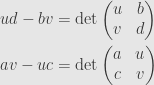
In other words, our solution is given by ratios of determinants:

and similar formulae hold for larger systems of equations.

The Hodge Star

Sorry for the delay from last Friday to today, but I was chasing down a good lead.

Anyway, last week I said that I’d talk about a linear map that extends the notion of the correspondence between parallelograms in space and perpendicular vectors.

First of all, we should see why there may be such a correspondence. We’ve identified -dimensional parallelepipeds in an -dimensional vector space with antisymmetric tensors of degree : . Of course, not every such tensor will correspond to a parallelepiped (some will be linear combinations that can’t be written as a single wedge of vectors), but we’ll just keep going and let our methods apply to such more general tensors. Anyhow, we also know how to count the dimension of the space of such tensors:

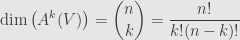
This formula tells us that and will have the exact same dimension, and so it makes sense that there might be an isomorphism between them. And we’re going to look for one which defines the “perpendicular” -dimensional parallelepiped with the same size.

So what do we mean by “perpendicular”? It’s not just in terms of the “angle” defined by the inner product. Indeed, in that sense the parallelograms and are perpendicular. No, we want any vector in the subspace defined by our parallelepiped to be perpendicular to any vector in the subspace defined by the new one. That is, we want the new parallelepiped to span the orthogonal complement to the subspace we start with.

Our definition will also need to take into account the orientation on . Indeed, considering the parallelogram in three-dimensional space, the perpendicular must be for some nonzero constant , or otherwise it won’t be perpendicular to the whole – plane. And has to be in order to get the right size. But will it be or ? The difference is entirely in the orientation.

Okay, so let’s pick an orientation on , which gives us a particular top-degree tensor so that . Now, given some , we define the Hodge dual to be the unique antisymmetric tensor of degree satisfying

for all . Notice here that if and describe parallelepipeds, and any side of is perpendicular to all the sides of , then the projection of onto the subspace spanned by will have zero volume, and thus . This is what we expect, for then this side of must lie within the perpendicular subspace spanned by , and so the wedge should also be zero.

As a particular example, say we have an orthonormal basis of so that . Then given a multi-index 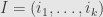the basic wedge gives us the subspace spanned by the vectors . The orthogonal complement is clearly spanned by the remaining basis vectors , and so , with the sign depending on whether the list 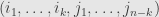is an even or an odd permutation of .

To be even more explicit, let’s work these out for the cases of dimensions three and four. First off, we have a basis . We work out all the duals of basic wedges as follows:

This reconstructs the correspondence we had last week between basic parallelograms and perpendicular basis vectors. In the four-dimensional case, the basis leads to the duals

It’s not a difficult exercise to work out the relation 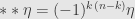for a degree tensor in an -dimensional space.