Today we conclude the proof of the classification theorem. The first four parts of the proof are here, here, here, and here.
- The only possible Coxeter graphs with a triple vertex are those of the forms
 ,
,  ,
,  , and
, and  .
.


From step 8 we have the labelled graph

Like we did in step 9, we define


These vectors  ,
,  , and
, and  are mutually orthogonal, linearly independent vectors, and that
  is not in the subspace that they span.
We look back at our proof of step 4 to determine that  ; where
  ,
,  , and
, and  are the angles between and , , and , respectively. We look back at our proof of step 9 to determine that
  ,
,  , and
, and  . Thus we can calculate the cosine

And similarly we find  , and
, and  . Adding up, we find
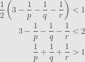
This last inequality, by the way, is hugely important in many areas of mathematics, and it’s really interesting to find it cropping up here.
Anyway, now none of  ,
,  , or
, or  can be
  or we don’t have a triple vertex at all. We can also choose which strand is which so that

We can determine from here that

and so we must have  , and the shortest leg must be one edge long. Now we have
  , and so
  , and must be either
  or
or  .
.
If  , then the second shortest leg is two edges long. In this case,
  and
and  . The possibilities for the triple
  are
are  ,
,  , and
, and  ; giving graphs , , and , respectively.
On the other hand, if  , then the second shortest leg is also one edge long. In this case, there is no more restriction on , and so the remaining leg can be as long as we like. This gives us the family of graphs.
And we’re done! If we have one triple edge, we must have the graph  . If we have a double edge or a triple vertex, we can have only one, and we can’t have one of each. Step 9 narrows down graphs with a double edge to
  and the families
  and
and  , while step 10 narrows down graphs with a triple vertex to , , and , and the family . Finally, if there are no triple vertices or double edges, we’re left with a single simple chain of type
  .
.
February 26, 2010
Posted by John Armstrong |
Geometry, Root Systems |
Leave a comment
We continue proving the classification theorem. The first three parts are here, here, and here.
- Any connected graph
 takes one of the four following forms: a simple chain, the graph, three simple chains joined at a central vertex, or a chain with exactly one double edge.
This step largely consolidates what we’ve done to this point. Here are the four possible graphs:


The labels will help with later steps.
Step 5 told us that there’s only one connected graph that contains a triple edge. Similarly, if we had more than one double edge or triple vertex, then we must be able to find two of them connected by a simple chain. But that will violate step 7, and so we can only have one of these features either.
- The only possible Coxeter graphs with a double edge are those underlying the Dynkin diagrams , , and .


Here we’ll use the labels on the above graph. We define


As in step 6, we find that  and all other pairs of vectors are orthogonal. And so we calculate
And similarly,  . We also know that
  , and so we find

Now we can use the Cauchy-Schwarz inequality to conclude that

where the inequality is strict, since and are linearly independent. And so we find

We thus must have either  , which gives us the diagram, or
  or
or  with the other arbitary, which give rise the the and Coxeter graphs.
February 25, 2010
Posted by John Armstrong |
Geometry, Root Systems |
5 Comments
Sorry, but what with errands today and work on some long-term plans, I forgot to put this post up this afternoon.
We continue with the proof of the classification theorem. The first two parts are here and here.
- If
 is a simple chain in the graph , then we can remove these vectors and replace them by their sum. The resulting set is still admissible, and its graph is obtained from by contracting the chain to a single vertex.
A simple chain in is a subgraph like
We define

I say that if we replace  by
by  in
in  then we still have an admissible set
  . Any edges connecting to any of the vertices
  will then connect to the vertex .
It should be clear that is still linearly independent. If there’s no way to write zero as a nontrivial linear combination of the vectors in , then of course there’s no way to do it with the additional condition that the coefficients of all the are the same.
Because we have a simple chain, we find  for
for  and
and  otherwise. Thus we calculate (compare to step 2)

and so is a unit vector.
Any  can be connected by an edge to at most one of the , or else would contain a cycle (violating step 3). Thus we have either
  if is connected to no vertex of the chain, or
  if is connected to by some number of edges. In either case we still find that
  is
is  , , , or , and so is admissible.
Further, the previous paragraph shows that the edges connecting to any other vertex of the graph are exactly the edges connecting the chain to . Thus we obtain the graph  of by contracting the chain in to a single vertex.
- The graph contains no subgraph of any of the following forms:


Indeed, if one of these graphs occurred in it would be (by step 1) the graph of an admissible set itself. However, if this were the case we could contract the central chain to a single vertex by step 6. We would then find one of the graphs


But each of these graphs has four edges incident on the central vertex, which violates step 4!
February 25, 2010
Posted by John Armstrong |
Geometry, Root Systems |
4 Comments
We continue with the proof of the classification theorem that we started yesterday.
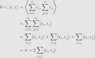
- No more than three edges (counting multiplicities) can be incident on any given vertex of .
Consider some vector  , and let
  be the vectors whose vertices are connected to by at least one edge. Since by step 3 the graph cannot contain any cycles, we cannot connect any
  and
and  , and so we have
  for
for  .
.
Since the collection  is linearly independent, there must be some unit vector
  in the span of these vectors which is perpendicular to each of the . This vector must satisfy
  . Then the collection
 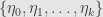 is an orthonormal basis of this subspace, and we can thus write
and thus

Now since we can’t have  , we must find

and thus

But  is the number of edges (counting multiplicities) between and , and so this sum is the total number of edges incident on .
- The only connected Coxeter graph containing a triple edge is
Indeed, step 4 tells us that no vertex can support more than three incident edges, counting multiplicities. Once we put the triple edge between two vertices, neither of them has any more room for another edge to connect to any other vertices. Thus the connected component cannot grow larger than this.
February 23, 2010
Posted by John Armstrong |
Geometry, Root Systems |
3 Comments
This week, we will prove the classification theorem for root systems. The proof consist of a long series of steps, and we’ll split it up over a number of posts.
Our strategy is to determine which Coxeter graphs can arise from actual root systems, and then see what Dynkin diagrams we can get. Since Coxeter graphs ignore relative lengths of roots, we will start by just working with unit vectors whose pairwise angles are described by the Coxeter graph.
So, for the time being we make the following assumptions:  is a real inner-product space (of arbitrary dimension), and
  is a set of
  linearly independent unit vectors satisfying
  and
and  is one of , , , or for . For the duration of this proof, we will call such a set of vectors “admissible”. The elements of a base
  for a root system
  , divided by their lengths, are an admissible set.
We construct a Coxeter graph , just as before, for every admissible set, and these clearly include the Coxeter graphs that come from root systems. Our task is now to classify all the connected Coxeter graphs that come from admissible sets of vectors.
- If we remove some of the vectors from an admissible set, then the remaining vectors still form an admissible set. The Coxeter graph of the new set is obtained from that of the old one by removing the vertices corresponding to the removed vectors and all their incident edges.
This should be straightforward. The remaining vectors are still linearly independent, and they still have unit length. The angles between each pair are also unchanged. All we do is remove some vectors (vertices in the graph).
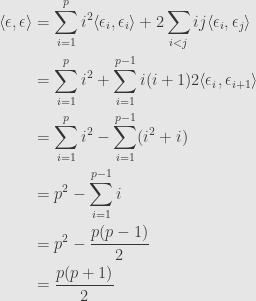
- The number of pairs of vertices in connected by at least one edge is strictly less than — the number of overall vertices.
Let us define

Since the are linearly independent, cannot be zero. Thus we find that
Now, for any pair and  joined by an edge, we must find that is , , or , and thus that
  . Clearly, we can have no more than
  of these edges if we are to satisfy the above inequality.
- The graph contains no cycles
Indeed, if we have a cycle of length in the graph, we could (using our step 1) discard all the vertices not involved in the cycle and still have the graph of an admissible set. But this graph would have vertices and at least edges — the ones involved in the cycle. But this is is impossible by step 2!
February 22, 2010
Posted by John Armstrong |
Geometry, Root Systems |
8 Comments
At long last, we can state the classification of irreducible root systems up to isomorphism. We’ve shown that for each such root system we can construct a connected Dynkin diagram, which determines a Cartan matrix, which determines the root system itself, up to isomorphism. So what he have to find now is a list of Dynkin diagrams which can possibly arise from a root system. And so today we state the
CLASSIFICATION THEOREM
If is an irreducible root system, then its Dynkin diagram is in one of four infinite families, or one of five “exceptional” diagrams. The four infinite families are
The  series. These consist of a single long string of roots with single edges connecting them. The diagrams are indexed by the number of roots, starting at
  :
:
The  series. These look like the series, except the last two roots are connected by a double edge, with the last root shorter. The diagrams are indexed by the number of roots, starting at
  :
:
The  series. These look like the series, except the last root is longer. The diagrams are indexed by the number of roots, starting at
  :
:
The  series. These look like the series, except the end is split into two roots. The diagrams are indexed by the number of roots, starting at
  :
:
The exceptional diagrams are
The  series. These have a string of roots connected by single edges. On the third root from the end of the string, a single edge branches off to another root on the side. The diagrams are indexed by the number of roots, for
  ,
,  , and
, and  :
:
The diagram. This consists of four roots in a row. The first two and last two are connected by a single edge, while the middle two are connected by a double edge:
- :
The diagram. This consists of two roots, connected by a triple edge:
- :
Our proof will take a number of steps, winnowing down the possible diagrams to this collection. We will spread it over the next week. But over the weekend, you can amuse yourself by working out the Cartan matrices for each of these Dynkin diagrams.
February 19, 2010
Posted by John Armstrong |
Geometry, Root Systems |
12 Comments
We’ve taken our root system and turned it into a Cartan matrix. Now we’re going to take our Cartan matrix and turn it into a pictorial form that we can really get our hands on.
Given a Cartan matrix, we want to construct a combinatorial graph. If the matrix is  , then we start with points. The rows and columns of the matrix correspond to simple roots, and so each of these points corresponds to a simple root as well. Noting this, we will call the points “roots”.
Now given any two simple roots  and
and  we can construct the Cartan integers
  and
and  . Our data about pairs of roots tells us that the product
  is either
  ,
,  ,
,  , or
, or  . We’ll connect each pair of roots by this many lines, like so:
The resulting combinatorial graph is called the “Coxeter graph” of This is almost enough information to recover the Cartan matrix. Unfortunately, in the two- and three-edge cases, we know that the two roots have different lengths, and we have no way of telling which is which. To fix this, we will draw an arrow (that looks suspiciously like a “greater-than” sign) pointing from the larger of the two roots to the smaller, like so:
In each case we know one root must be longer than the other, and by a particular ratio. And so with this information we call the graph a “Dynkin diagram”, and it is enough to reconstruct the Cartan matrix. For example, consider the Dynkin diagram called :
We can use this to reconstruct the Cartan matrix:

One nice thing about Dynkin diagrams is that we really don’t care about the order of the roots, like we had to do for the Cartan matrix. They also show graphically a lot of information about the root system. For instance, we may be able to break a Dynkin diagram up into more than one connected component. Any root in one of these components has no edges connecting it to a root in another. This means that  , and thus that and are perpendicular. This breaks the base up into a bunch of mutually-perpendicular subsets, which give rise to irreducible components of the root system .
The upshot of this last fact is that irreducibility of a root system corresponds to connectedness of its Dynkin diagram. Thus our project has come down to this question: which connected Dynkin diagrams arise from root systems? At last, we’re almost ready to answer this question.
February 18, 2010
Posted by John Armstrong |
Geometry, Root Systems |
10 Comments
Yesterday, we showed that a Cartan matrix determines its root system up to isomorphism. That is, in principle if we have a collection of simple roots and the data about how each projects onto each other, that is enough to determine the root system itself. Today, we will show how to carry this procedure out.
But first, we should point out what we don’t know: which Cartan matrices actually come from root systems! We know some information, though. First off, the diagonal entries must all be . Why? Well, it’s a simple calculation to see that for any vector

The off-diagonal entries, on the other hand, must all be negative or zero. Indeed, our simple roots must be part of a base , and any two vectors  must satisfy
  . Even better, we have a lot of information about pairs of roots. If one off-diagonal
  element is zero, so must the corresponding one
  on the other side of the diagonal be zero. And if they’re nonzero, we have a very tightly controlled number of options. One must be
  , and the other must be ,
  , or
, or  .
.
But beyond that, we don’t know which Cartan matrices actually arise, and that’s the whole point of our project. For now, though, we will assume that our matrix does in fact arise from a real root system, and see how to use it to construct a root system whose Cartan matrix is the given one. And our method will hinge on considering root strings.
What we really need is to build up all the positive roots  , and then the negative roots
  will just be a reflected copy of . We also know that since there are only finitely many roots, there can be only finitely many heights, and so there is some largest height. And we know that we can get to any positive root of any height by adding more and more simple roots. So we will proceed by building up all the roots of height , then height , and so on until we cannot find any higher roots, at which point we will be done.
So let’s start with roots of height . These are exactly the simple roots, and we are just given those to begin with. We know all of them, and we know that there is nothing at all below them (among positive roots, at least).
Next we come to the roots of height . Every one of these will be a root of height plus another simple root. The problem is that we can’t add just any simple root to a root of height to get another root of height . If we step in the wrong direction we’ll fall right off the root system! We need to know which directions are safe, and that’s where root strings come to the rescue. We start with a root with  , and a simple root . We know that the length of the string through must be . But we also know that we can’t step backwards, because
  would be (in this case) a linear combination of simple roots with both positive and negative coefficients! If
  then we can’t step forwards either, because we’ve already got the whole root string. But if
  then we have room to take a step in the direction from , giving a root
  with height
  . As we repeat this over all roots of height and all simple roots , we must eventually cover all of the roots of height .
Next are the roots of height . Every one of these will be a root of height plus another simple root. The problem is that we can’t add just any simple root to a root of height to get another root of height . If we step in the wrong direction we’ll fall right off the root system! We need to know which directions are safe, and that’s where root strings come to the rescue… again. We start with a root with  , and a simple root . We know that the length of the string through must again be . But now we may be able to take a step backwards! That is, it may turn out that is a root, and that complicates matters. But this is okay, because if is a root, then it must be of height , and we know that we already know all of these! So, look up in our list of roots of height and see if it shows up. If it doesn’t, then the string through
  starts at , just like before. If it does show up, then the root string must start at . Indeed, if we took another step backwards, we’ve have a root of height , which doesn’t exist. Thus we know where the root string starts. We can also tell how long it is, because we can calculate by adding up the Cartan integers
  for each of the simple roots
  we’ve used to build . And so we can tell whether or not it’s safe to take another step in the direction of from , and in this way we can build up each and every root of height .
And so on at each level we start with the roots of height and look from each one in the direction of each simple root . In each case, we can carefully step backwards to determine where the string through begins, and we can calculate the length of the string, and so we can tell whether or not it’s safe to take another step in the direction of from , and we can build up each and every root of height  . Of course, it may just happen (and eventually it must happen) that we find no roots of height . At this point, there can be no roots of any larger height either, and we’re done. We’ve built up all the positive roots, and the negative roots are just their negatives.
February 17, 2010
Posted by John Armstrong |
Geometry, Root Systems |
6 Comments
As we move towards our goal of classifying root systems, we find new ways of encoding the information contained in a root system . First comes the Cartan matrix.
Pick a base  of the root system. Since is finite-dimensional and is a basis of , must be finite, and so there’s no difficulty in picking some fixed order on the simple roots. That is, we write
 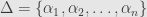 where
where  . Now we can define the “Cartan matrix” as the matrix whose entry in the
  th row and
  th column is . These entries are called “Cartan integers”.
The matrix we get, depends on the particular ordering of the base we chose, of course, so the Cartan matrix isn’t quite uniquely determined by the root system. This is relatively unimportant, actually. More to the point is the other direction: the Cartan matrix determines the root system up to isomorphism!
That is, let’s say  is another root system
  in another vector space with another identified base
  . Further, assume that for all
  we have
 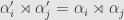 , so the Cartan matrix determined by
  is equal to the Cartan matrix determined by . I say that the bijection
  extends to an isomorphism
  that sends onto and satisfies
  for all roots
  .
.
The unique extension to  is trivial. Indeed, since is a basis for all we have to do is specify all the images
  and there is a unique linear transformation extending the mapping on basis vectors. And it’s an isomorphism, since the image of our basis of is itself a basis of
  , so we can turn around and reverse everything.
Now our hypothesis that the bases give rise to the same Cartan matrix allows us to calculate for simple roots :

That is, intertwines the actions of each of the simple reflections  . But we know that the simple reflections with respect to any given base generate the Weyl group!
And so must intertwine the actions of the Weyl groups  and
and  . That is, the mapping
  is an isomorphism
  which sends to
  for all
  .
.
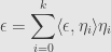
We can go further. Each root is in the -orbit of some simple root . Say  for . Then we find

And so must send to . A straightforward calculation (unwinding the one before) shows that must then preserve the Cartan integers for any roots and .
February 16, 2010
Posted by John Armstrong |
Geometry, Root Systems |
8 Comments
Today, I’d like to show you some examples of two-dimensional root systems, which illustrate a lot of what we talked about last week. I’ve worked them up in a Java application called Geogebra, but I don’t seem to be able to embed the resulting applets into a WordPress post. If someone knows how, I’d be glad to hear it.
Anyhow, in lieu of embedded applets, I’ll post the “.ggb” files, which you can take over to the Geogebra site and load up there. So, with no further ado, I present all four two-dimensional root systems:
Each one of these files illustrates the root system and its Weyl orbit. Each one has two simple roots, labelled and in blue. The rest of the roots are shown in black, and the fundamental domain is marked out by two rays perpendicular to and , respectively.
An arbitrary blue vector  is shown, along with its reflected images making up the entire Weyl orbit. You can grab this vector and drag it around, watching how the orbit changes. No matter where you place , notice that there is exactly one image in the fundamental domain, as we showed.
The first root system is reducible, but the other three are irreducible. For each of these, we can see that there is a unique maximal root. However,  doesn’t; both and are maximal.
We also see that the Weyl orbit of a root spans the plane in the irreducible cases. But, again, in the Weyl orbits of and only span their lines.
Finally, in each of the irreducible cases we see that there are at most two distinct root lengths. And, in each case, the unique maximal root is the long root within the fundamental domain.
February 15, 2010
Posted by John Armstrong |
Geometry, Root Systems |
3 Comments
:

:

:

:

:

:


:

:

:

:

:

:

:

:

:


:

:

:

:

:

:

:

:


