Hom-Space Additivity

Today I’d like to show that the space of homomorphisms between two -modules is “additive”. That is, it satisfies the isomorphisms:

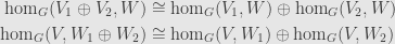
We should be careful here: the direct sums inside the are direct sums of -modules, while those outside are direct sums of vector spaces.

The second of these is actually the easier. If is a -morphism, then we can write it as , where and . Indeed, just take the projection 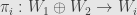and compose it with to get . These projections are also -morphisms, since and are -submodules. Since every can be uniquely decomposed, we get a linear map .

Then the general rules of direct sums tell us we can inject and back into , and write

Thus given any -morphisms and we can reconstruct an . This gives us a map in the other direction — — which is clearly the inverse of the first one, and thus establishes our isomorphism.

Now that we’ve established the second isomorphism, the first becomes clearer. Given a -morphism 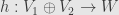we need to find morphisms . Before we composed with projections, so this time let’s compose with injections! Indeed, composes with to give 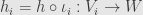. On the other hand, given morphisms , we can use the projections and compose them with the to get two morphisms . Adding them together gives a single morphism, and if the came from an , then this reconstructs the original. Indeed:

And so the first isomorphism holds as well.

We should note that these are not just isomorphisms, but “natural” isomorphisms. That the construction is a functor is clear, and it’s straightforward to verify that these isomorphisms are natural for those who are interested in the category-theoretic details.

Schur’s Lemma

Now that we know that images and kernels of –morphisms between –modules are -modules as well, we can bring in a very general result.

Remember that we call a -module irreducible or “simple” if it has no nontrivial submodules. In general, an object in any category is simple if it has no nontrivial subobjects. If a morphism in a category has a kernel and an image — as we’ve seen all -morphisms do — then these are subobjects of the source and target objects.

So now we have everything we need to state and prove Schur’s lemma. Working in a category where every morphism has both a kernel and an image, if is a morphism between two simple objects, then either is an isomorphism or it’s the zero morphism from to . Indeed, since is simple it has no nontrivial subobjects. The kernel of is a subobject of , so it must either be itself, or the zero object. Similarly, the image of must either be itself or the zero object. If either or then is the zero morphism. On the other hand, if and we have an isomorphism.

To see how this works in the case of -modules, every time I say “object” in the preceding paragraph replace it by “-module”. Morphisms are -morphisms, the zero morphism is the linear map sending every vector to , and the zero object is the trivial vector space . If it feels more comfortable, walk through the preceding proof making the required substitutions to see how it works for -modules.

In terms of matrix representations, let’s say and are two irreducible matrix representations of , and let be any matrix so that for all . Then Schur’s lemma tells us that either is invertible — it’s the matrix of an isomorphism — or it’s the zero matrix.

Stone Spaces

The Stone space functor we’ve been working with sends Boolean algebras to topological spaces. Specifically, it sends them to compact Hausdorff spaces. There’s another functor floating around, of course, though it might not be the one you expect.

The clue is in our extended result. Given a topological space we define to be the Boolean algebra of all clopen subsets. This functor is contravariant — given a continuous map , we get a homomorphism of Boolean algebras sending the clopen set to its preimage . It’s straightforward to see that this preimage is clopen. Another surprise is that this is known as the “Stone functor”, not to be confused with the Stone space functor .

So what happens when we put these two functors together? If we start with a Boolean algebra and build its Stone space , then the Stone functor applied to this space gives us a Boolean algebra . This is, by construction, isomorphic to itself. Thus the category is contravariantly equivalent to some subcategory of . But which compact Hausdorff spaces arise as the Stone spaces of Boolean algebras?

Look at the other composite; starting with a topological space , we find the Boolean algebra of its clopen subsets, and then the Stone space of this Boolean algebra. We also get a function . For each point we define the Boolean algebra homomorphism that sends a clopen set to if and only if . We can see that this is a continuous map by checking that the preimage of any basic set is open. Indeed, a basic set of is for some clopen set . That is, . Which functions of the form are in ? Exactly those for which . Since is clopen, this preimage is open.

Two points and are sent to the same function if and only if every clopen set containing also contains , and vice versa. That is, and must be in the same connected component. Indeed, if they were in different connected components, then there would be some clopen containing one but not the other. Conversely, if there is a clopen that contains one but not the other they can’t be in the same connected component. Thus this map collapses all the connected components of into points of .

If this map is a homeomorphism, then no two points of are in the same connected component. Thus each singleton is a connected component, and we call the space “totally disconnected”. Clearly, such a space is in the image of the Stone space functor. On the other hand, if , then , and so this is both a necessary and a sufficient condition. Thus the “Stone spaces” form the full subcategory of , consisting of the totally disconnected compact Hausdorff spaces. Stone’s representation theorem shows us that this category is equivalent to the dual of the category of Boolean algebras.

As a side note: I’d intended to cover the Stone-Čech compactification, but none of the references I have at hand actually cover the details. There’s a certain level below which everyone seems to simply assert certain facts and take them as given, and I can’t seem to reconstruct them myself.

Coproduct Root Systems

We should also note that the category of root systems has binary (and thus finite) coproducts. They both start the same way: given root systems and in inner-product spaces and , we take the direct sum of the vector spaces, which makes vectors from each vector space orthogonal to vectors from the other one.

The coproduct root system consists of the vectors of the form for and for . Indeed, this collection is finite, spans , and does not contain . The only multiples of any given vector in are that vector and its negative. The reflection sends vectors coming from to each other, and leaves vectors coming from fixed, and similarly for the reflection . Finally,

All this goes to show that actually is a root system. As a set, it’s the disjoint union of the two sets of roots.

As a coproduct, we do have the inclusion morphisms and , which are inherited from the direct sum of and . This satisfies the universal condition of a coproduct, since the direct sum does. Indeed, if is another root system, and if and are linear transformations sending and into , respectively, then sends into , and is the unique such transformation compatible with the inclusions.

Interestingly, the Weyl group of the coproduct is the product of the Weyl groups. Indeed, for every generator of and every generator of we get a generator . And the two families of generators commute with each other, because each one only acts on the one summand.

On the other hand, there are no product root systems in general! There is only one natural candidate for that would be compatible with the projections and . It’s made up of the points for and . But now we must consider how the projections interact with reflections, and it isn’t very pretty.

The projections should act as intertwinors. Specifically, we should have

and similarly for the other projection. In other words

But this isn’t a reflection! Indeed, each reflection has determinant , and this is the composition of two reflections (one for each component) so it has determinant . Thus it cannot be a reflection, and everything comes crashing down.

That all said, the Weyl group of the coproduct root system is the product of the two Weyl groups, and many people are mostly concerned with the Weyl group of symmetries anyway. And besides, the direct sum is just as much a product as it is a coproduct. And so people will often write even though it’s really not a product. I won’t write it like that here, but be warned that that notation is out there, lurking.

Functoriality of Tensor Algebras

The three constructions we’ve just shown — the tensor, symmetric tensor, and exterior algebras — were all asserted to be the “free” constructions. This makes them functors from the category of vector spaces over to appropriate categories of -algebras, and that means that they behave very nicely as we transform vector spaces, and we can even describe exactly how nicely with explicit algebra homomorphisms. I’ll work through this for the exterior algebra, since that’s the one I’m most interested in, but the others are very similar.

Okay, we want the exterior algebra to be the “free” graded-commutative algebra on the vector space . That’s a tip-off that we’re thinking should be the left adjoint of the “forgetful” functor which sends a graded-commutative algebra to its underlying vector space (Todd makes a correction to which forgetful functor we’re using below). We’ll define this adjunction by finding a collection of universal arrows, which (along with the forgetful functor ) is one of the many ways we listed to specify an adjunction.

So let’s run down the checklist. We’ve got the forgetful functor which we’re going to make the right-adjoint. Now for each vector space we need a graded-commutative algebra — clearly the one we’ll pick is — and a universal arrow . The underlying vector space of the exterior algebra is the direct sum of all the spaces of antisymmetric tensors on .

Yesterday we wrote this without the , since we often just omit forgetful functors, but today we want to remember that we’re using it. But we know that , so the obvious map to use is the one that sends a vector to itself, now considered as an antisymmetric tensor with a single tensorand.

But is this a universal arrow? That is, if is another graded-commutative algebra, and is another linear map, then is there a unique homomorphism of graded-commutative algebras so that ? Well, tells us where in we have to send any antisymmetric tensor with one tensorand. Any other element in is the sum of a bunch of terms, each of which is the wedge of a bunch of elements of . So in order for to be a homomorphism of graded-commutative algebras, it has to act by simply changing each element of in our expression for into the corresponding element of , and then wedging and summing these together as before. Just write out the exterior algebra element all the way down in terms of vectors, and transform each vector in the expression. This will give us the only possible such homomorphism . And this establishes that is the object-function of a functor which is left-adjoint to .

So how does work on morphisms? It’s right in the proof above! If we have a linear map , we need to find some homomorphism . But we can compose with the linear map , which gives us . The universality property we just proved shows that we have a unique homomorphism . And, specifically, it is defined on an element by writing down in terms of vectors in and applying to each vector in the expression to get a sum of wedges of elements of , which will be an element of the algebra .

Of course, as stated above, we get similar constructions for the commutative algebra and the tensor algebra .

Since, given a linear map the induced homomorphisms , , and preserve the respective gradings, they can be broken into one linear map for each degree. And if is invertible, so must be its image under each functor. These give exactly the tensor, symmetric, and antisymmetric representations of the group , if we consider how these functors act on invertible morphisms . Functoriality is certainly a useful property.

Galois Connections

I want to mention a topic I thought I’d hit back when we talked about adjoint functors. We know that every poset is a category, with the elements as objects and a single arrow from to if . Functors between such categories are monotone functions, preserving the order. Contravariant functors are so-called “antitone” functions, which reverse the order, but the same abstract nonsense as usual tells us this is just a monotone function to the “opposite” poset with the order reversed.

So let’s consider an adjoint pair of such functors. This means there is a natural isomorphism between and . But each of these hom-sets is either empty (if ) or a singleton (if ). So the adjunction between and means that if and only if . The analogous condition for an antitone adjoint pair is that if and only if .

There are some immediate consequences to having a Galois connection, which are connected to properties of adjoints. First off, we know that and . This essentially expresses the unit and counit of the adjunction. For the antitone version, let’s show the analogous statement more directly: we know that , so the adjoint condition says that . Similarly, . This second condition is backwards because we’re reversing the order on one of the posets.

Using the unit and the counit of an adjunction, we found a certain quasi-inverse relation between some natural transformations on functors. For our purposes, we observe that since we have the special case . But , and preserves the order. Thus . So . Similarly, we find that , which holds for both monotone and antitone Galois connections.

Chasing special cases further, we find that , and that for either kind of Galois connection. That is, and are idempotent functions. In general categories, the composition of two adjoint functors gives a monad, and this idempotence is just the analogue in our particular categories. In particular, these functions behave like closure operators, but for the fact that general posets don’t have joins or bottom elements to preserve in the third and fourth Kuratowski axioms.

And so elements left fixed by (or ) are called “closed” elements of the poset. The images of and consist of such closed elements

The Category of Representations of a Group

Sorry for missing yesterday. I had this written up but completely forgot to post it while getting prepared for next week’s trip back to a city. Speaking of which, I’ll be heading off for the week, and I’ll just give things here a rest until the beginning of December. Except for the Samples, and maybe an I Made It or so…

Okay, let’s say we have a group . This gives us a cocommutative Hopf algebra. Thus the category of representations of is monoidal — symmetric, even — and has duals. Let’s consider these structures a bit more closely.

We start with two representations and . We use the comultiplication on to give us an action on the tensor product . Specifically, we find

That is, we make two copies of the group element , use to act on the first tensorand, and use to act on the second tensorand. If and came from actions of on sets, then this is just what you’d expect from linearizing the product of the -actions.

Symmetry is straightforward. We just use the twist on the underlying vector spaces, and it’s automatically an intertwiner of the actions, so it defines a morphism between the representations.

Duals, though, take a bit of work. Remember that the antipode of sends group elements to their inverses. So if we start with a representation we calculate its dual representation on :

Composing linear maps from the right reverses the order of multiplication from that in the group, but taking the inverse of reverses it again, and so we have a proper action again.

Cocommutativity

One things I don’t think I’ve mentioned is that the category of vector spaces over a field is symmetric. Indeed, given vector spaces and we can define the “twist” map by setting and extending linearly.

Now we know that an algebra is commutative if we can swap the inputs to the multiplication and get the same answer. That is, if . Or, more succinctly: .

Reflecting this concept, we say that a coalgebra is cocommutative if we can swap the outputs from the comultiplication. That is, if . Similarly, bialgebras and Hopf algebras can be cocommutative.

The group algebra of a group is a cocommutative Hopf algebra. Indeed, since , we can twist this either way and get the same answer.

So what does cocommutativity buy us? It turns out that the category of representations of a cocommutative bialgebra is not only monoidal, but it’s also symmetric! Indeed, given representations and , we have the tensor product representations on , and on . To twist them we define the natural transformation to be the twist of the vector spaces: .

We just need to verify that this actually intertwines the two representations. If we act first and then twist we find

On the other hand, if we twist first and then act we find

It seems there’s a problem. In general this doesn’t work. Ah! but we haven’t used cocommutativity yet! Now we write

Again, remember that this doesn’t mean that the two tensorands are always equal, but only that the results after (implicitly) summing up are equal. Anyhow, that’s enough for us. It shows that the twist on the underlying vector spaces actually does intertwine the two representations, as we wanted. Thus the category of representations is symmetric.

The Category of Representations of a Hopf Algebra

It took us two posts, but we showed that the category of representations of a Hopf algebra has duals. This is on top of our earlier result that the category of representations of any bialgebra is monoidal. Let’s look at this a little more conceptually.

Earlier, we said that a bialgebra is a comonoid object in the category of algebras over . But let’s consider this category itself. We also said that an algebra is a category enriched over , but with only one object. So we should really be thinking about the category of algebras as a full sub-2-category of the 2-category of categories enriched over .

So what’s a comonoid object in this 2-category? When we defined comonoid objects we used a model category . Now let’s augment it to a 2-category in the easiest way possible: just add an identity 2-morphism to every morphism!

But the 2-category language gives us a bit more flexibility. Instead of demanding that the morphism satisfy the associative law on the nose, we can add a “coassociator” 2-morphism to our model 2-category. Similarly, we dispense with the left and right counit laws and add left and right counit 2-morphisms. Then we insist that these 2-morphisms satisfy pentagon and triangle identities dual to those we defined when we talked about monoidal categories.

What we’ve built up here is a model 2-category for weak comonoid objects in a 2-category. Then any weak comonoid object is given by a 2-functor from this 2-category to the appropriate target 2-category. Similarly we can define a weak monoid object as a 2-functor from the opposite model 2-category to an appropriate target 2-category.

So, getting a little closer to Earth, we have in hand a comonoid object in the 2-category of categories enriched over — our algebra . But remember that a 2-category is just a category enriched over categories. That is, between (considered as a category) and we have a hom-category . The entry in the first slot is described by a 2-functor from the model category of weak comonoid objects to the 2-category of categories enriched over . This hom-functor is contravariant in the first slot (like all hom-functors), and so the result is described by a 2-functor from the opposite of our model 2-category. That is, it’s a weak monoid object in the 2-category of all categories. And this is just a monoidal category!

This is yet another example of the way that hom objects inherit structure from their second variable, and inherit opposite structure from their first variable. I’ll leave it to you to verify that a monoidal category with duals is similarly a weak group object in the 2-category of categories, and that this is why a Hopf algebra — a (weak) cogroup object in the 2-category of categories enriched over has dual representations.

Representations of Hopf Algebras II

Now that we have a coevaluation for vector spaces, let’s make sure that it intertwines the actions of a Hopf algebra. Then we can finish showing that the category of representations of a Hopf algebra has duals.

Take a representation , and pick a basis of and the dual basis of . We define the map by . Now , so if we use the action of on before transferring to , we get . Be careful not to confuse the counit with the basis elements .

On the other hand, if we transfer first, we must calculate

Now let’s use the fact that we’ve got this basis sitting around to expand out both and as matrices. We’ll just take on matrix indices on the right for our notation. Then we continue the calculation above:

And so the coevaluation map does indeed intertwine the two actions of . Together with the evaluation map, it provides the duality on the category of representations of a Hopf algebra that we were looking for.