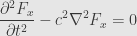
We’ve derived a “wave equation” from Maxwell’s equations, but it’s not clear what it means, or even why this is called a wave equation. Let’s consider the abstracted form, which both electric and magnetic fields satisfy:

where  is the “Laplacian” operator, defined on scalar functions by taking the gradient followed by the divergence, and extended linearly to vector fields. If we have a Cartesian coordinate system — and remember we’re working in good, old
  so it’s possible to pick just such coordinates, albeit not canonically — we can write
where  is the
  -component of
  , and a similar equation holds for the
  and
and  components as well. We can also write out the Laplacian in terms of coordinate derivatives:
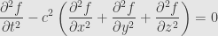
Let’s simplify further to just consider functions that depend on and  , and which are constant in the and directions:
![\displaystyle\frac{\partial^2f}{\partial t^2}-c^2\frac{\partial^2f}{\partial x^2}=\left[\frac{\partial^2}{\partial t^2}-c^2\frac{\partial^2}{\partial x^2}\right]f=0](https://s0.wp.com/latex.php?latex=%5Cdisplaystyle%5Cfrac%7B%5Cpartial%5E2f%7D%7B%5Cpartial+t%5E2%7D-c%5E2%5Cfrac%7B%5Cpartial%5E2f%7D%7B%5Cpartial+x%5E2%7D%3D%5Cleft%5B%5Cfrac%7B%5Cpartial%5E2%7D%7B%5Cpartial+t%5E2%7D-c%5E2%5Cfrac%7B%5Cpartial%5E2%7D%7B%5Cpartial+x%5E2%7D%5Cright%5Df%3D0&bg=e6e6e6&fg=333333&s=0&c=20201002)
We can take this big operator and “factor” it:
![\displaystyle\left[\left(\frac{\partial}{\partial t}+c\frac{\partial}{\partial x}\right)\left(\frac{\partial}{\partial t}-c\frac{\partial}{\partial x}\right)\right]f=0](https://s0.wp.com/latex.php?latex=%5Cdisplaystyle%5Cleft%5B%5Cleft%28%5Cfrac%7B%5Cpartial%7D%7B%5Cpartial+t%7D%2Bc%5Cfrac%7B%5Cpartial%7D%7B%5Cpartial+x%7D%5Cright%29%5Cleft%28%5Cfrac%7B%5Cpartial%7D%7B%5Cpartial+t%7D-c%5Cfrac%7B%5Cpartial%7D%7B%5Cpartial+x%7D%5Cright%29%5Cright%5Df%3D0&bg=e6e6e6&fg=333333&s=0&c=20201002)
Any function which either “factor” sends to zero will be a solution of the whole equation. We find solutions like
![\displaystyle\begin{aligned}\left[\frac{\partial}{\partial t}+c\frac{\partial}{\partial x}\right]A(x-ct)&=A'(x-ct)\frac{\partial(x-ct)}{\partial t}+cA'(x-ct)\frac{\partial(x-ct)}{\partial x}\\&=A'(x-ct)(-c+c)=0\\\left[\frac{\partial}{\partial t}-c\frac{\partial}{\partial x}\right]B(x+ct)&=B'(x+ct)\frac{\partial(x+ct)}{\partial t}-cB'(x+ct)\frac{\partial(x+ct)}{\partial x}\\&=B'(x+ct)(c-c)=0\end{aligned}](https://s0.wp.com/latex.php?latex=%5Cdisplaystyle%5Cbegin%7Baligned%7D%5Cleft%5B%5Cfrac%7B%5Cpartial%7D%7B%5Cpartial+t%7D%2Bc%5Cfrac%7B%5Cpartial%7D%7B%5Cpartial+x%7D%5Cright%5DA%28x-ct%29%26%3DA%27%28x-ct%29%5Cfrac%7B%5Cpartial%28x-ct%29%7D%7B%5Cpartial+t%7D%2BcA%27%28x-ct%29%5Cfrac%7B%5Cpartial%28x-ct%29%7D%7B%5Cpartial+x%7D%5C%5C%26%3DA%27%28x-ct%29%28-c%2Bc%29%3D0%5C%5C%5Cleft%5B%5Cfrac%7B%5Cpartial%7D%7B%5Cpartial+t%7D-c%5Cfrac%7B%5Cpartial%7D%7B%5Cpartial+x%7D%5Cright%5DB%28x%2Bct%29%26%3DB%27%28x%2Bct%29%5Cfrac%7B%5Cpartial%28x%2Bct%29%7D%7B%5Cpartial+t%7D-cB%27%28x%2Bct%29%5Cfrac%7B%5Cpartial%28x%2Bct%29%7D%7B%5Cpartial+x%7D%5C%5C%26%3DB%27%28x%2Bct%29%28c-c%29%3D0%5Cend%7Baligned%7D&bg=e6e6e6&fg=333333&s=0&c=20201002)
where  and
and  are pretty much any function that’s at least mildly well-behaved.
We call solutions of the first form “right-moving”, for if we view as time and watch as it increases, the “shape” of  stays the same; it just moves in the increasing direction. That is, at time
  we see the same thing at that we saw at
  —
—  units to the left — at time
  . Similarly, we call solutions of the second form “left-moving”. In each family, solutions propagate at a rate of
  , which was the constant from our original equation. Any solution of this simplified, one-dimensional wave equation will be the sum of a right-moving and a left-moving term.
More generally, for the three-dimensional version we have “plane-wave” solutions propagating in any given direction we want. We could do a big, messy calculation, but note that if  is any unit vector, we can pick a Cartesian coordinate system where is the unit vector in the direction, in which case we’re back to the right-moving solutions from above. And of course there’s no reason we can’t let be a vector-valued function. Such a solution looks like

The bigger is, the further in the direction the position vector  must extend to compensate; the shape
  stays the same, but moves in the direction of with a velocity of .
It will be helpful to work out some of the basic derivatives of such solutions. Time is easy:
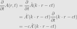
Spatial derivatives are a little trickier. We pick a Cartesian coordinate system to write:

We don’t really want to depend on coordinates, so luckily it’s easy enough to figure out:

which will make our lives much easier to have worked out in advance.
February 8, 2012
Posted by John Armstrong |
Analysis, Differential Equations |
3 Comments
Now that we’ve got the existence and uniqueness of our solutions down, we have one more of our promised results: the smooth dependence of solutions on initial conditions. That is, if we use our existence and uniqueness theorems to construct a unique “flow” function 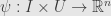 satisfying

by setting 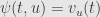 — where
  is the unique solution with initial condition
  — then
  is continuously differentiable.
Now, we already know that is continuously differentiable in the time direction by definition. What we need to show is that the directional derivatives involving directions in  exist and are continuous. To that end, let
  be a base point and
  be a small enough displacement that
  as well. Similarly, let be a fixed point in time and let
  be a small change in time

But now our result from last time tells us that these solutions can diverge no faster than exponentially. Thus we conclude that

and so as  this term must go to zero as well. Meanwhile, the second term also goes to zero by the differentiability of
  . We can now see that the directional derivative at
  in the direction of
  exists.
But are these directional derivatives continuous. This turns out to be a lot more messy, but essentially doable by similar methods and a generalization of Gronwall’s inequality. For the sake of getting back to differential equations I’m going to just assert that not only do all directional derivatives exist, but they’re continuous, and thus the flow is  .
.
May 16, 2011
Posted by John Armstrong |
Analysis, Differential Equations |
Leave a comment
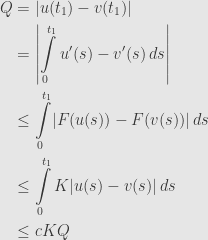
Now we can establish some control on how nearby solutions to the differential equation

diverge. That is, as time goes by, how can the solutions move apart from each other?
Let and be two solutions satisfying initial conditions  and
and  , respectively. The existence and uniqueness theorems we’ve just proven show that and are uniquely determined by this choice in some interval, and we’ll pick a
  so they’re both defined on the closed interval
 ![[t_0,t_1]](https://s0.wp.com/latex.php?latex=%5Bt_0%2Ct_1%5D&bg=e6e6e6&fg=333333&s=0&c=20201002) . Now for every in this interval we have
. Now for every in this interval we have

Where  is a Lipschitz constant for in the region we’re concerned with. That is, the separation between the solutions
  and
and  can increase no faster than exponentially.
So, let’s define  to be this distance. Converting to integral equations, it’s clear that
and thus
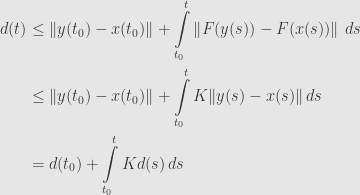
Now Gronwall’s inequality tells us that  , which is exactly the inequality we asserted above.
May 13, 2011
Posted by John Armstrong |
Analysis, Differential Equations |
1 Comment
We’re going to need another analytic lemma, this one called “Gronwall’s inequality”. If ![v:[0,\alpha]\to\mathbb{R}](https://s0.wp.com/latex.php?latex=v%3A%5B0%2C%5Calpha%5D%5Cto%5Cmathbb%7BR%7D&bg=e6e6e6&fg=333333&s=0&c=20201002) is a continuous, nonnegative function, and if
is a continuous, nonnegative function, and if  and are nonnegative constants such that
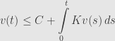
for all ![t\in[0,\alpha]](https://s0.wp.com/latex.php?latex=t%5Cin%5B0%2C%5Calpha%5D&bg=e6e6e6&fg=333333&s=0&c=20201002) then for all in this interval we have
then for all in this interval we have

That is, we can conclude that  grows no faster than an exponential function. Exponential growth may seem fast, but at least it doesn’t blow up to an infinite singularity in finite time, no matter what Kurzweil seems to think.
Anyway, first let’s deal with strictly positive . If we define

then by assumption we have  . Differentiating, we find
  , and thus

Integrating, we find

Finally we can exponentiate to find

proving Gronwall’s inequality.
If  , in our hypothesis, the hypothesis is true for any
  in its place, and so we see that
  for any positive
  , which means that
  must be zero, as required by Gronwall’s inequality in this case.
May 11, 2011
Posted by John Armstrong |
Analysis, Differential Equations |
3 Comments
I’d like to go back and give a different proof that the Picard iteration converges — one which is closer to the spirit of Newton’s method. In that case, we proved that Newton’s method converged by showing that the derivative of the iterating function was less than one at the desired solution, making it an attracting fixed point.
In this case, however, we don’t have a derivative because our iteration runs over functions rather than numbers. We will replace it with a similar construction called the “functional derivative”, which is a fundamental part of the “calculus of variations”. I’m not really going to go too deep into this field right now, and I’m not going to prove the analogous result that a small functional derivative means an attracting fixed point, but it’s a nice exercise and introduction anyway.
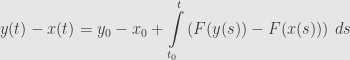
So, we start with the Picard iteration again:
=a+\int\limits_0^tF(v(s))\,ds](https://s0.wp.com/latex.php?latex=%5Cdisplaystyle+P%5Bv%5D%28t%29%3Da%2B%5Cint%5Climits_0%5EtF%28v%28s%29%29%5C%2Cds&bg=e6e6e6&fg=333333&s=0&c=20201002)
We consider what happens when we add an adjustment to :
&=a+\int\limits_0^tF(v(s)+h(s))\,ds\\&\approx a+\int\limits_0^tF(v(s))+dF(v(s))h(s)\,ds\\&=a+\int\limits_0^tF(v(s))\,ds+\int\limits_0^tdF(v(s))h(s)\,ds\\&=P[v](t)+\int\limits_0^tdF(v(s))h(s)\,ds\end{aligned}](https://s0.wp.com/latex.php?latex=%5Cdisplaystyle%5Cbegin%7Baligned%7DP%5Bv%2Bh%5D%28t%29%26%3Da%2B%5Cint%5Climits_0%5EtF%28v%28s%29%2Bh%28s%29%29%5C%2Cds%5C%5C%26%5Capprox+a%2B%5Cint%5Climits_0%5EtF%28v%28s%29%29%2BdF%28v%28s%29%29h%28s%29%5C%2Cds%5C%5C%26%3Da%2B%5Cint%5Climits_0%5EtF%28v%28s%29%29%5C%2Cds%2B%5Cint%5Climits_0%5EtdF%28v%28s%29%29h%28s%29%5C%2Cds%5C%5C%26%3DP%5Bv%5D%28t%29%2B%5Cint%5Climits_0%5EtdF%28v%28s%29%29h%28s%29%5C%2Cds%5Cend%7Baligned%7D&bg=e6e6e6&fg=333333&s=0&c=20201002)
We call the small change the “variation” of , and we write  . Similarly, we call the difference between
 ![P[v+\delta v]](https://s0.wp.com/latex.php?latex=P%5Bv%2B%5Cdelta+v%5D&bg=e6e6e6&fg=333333&s=0&c=20201002) and
and ![P[v]](https://s0.wp.com/latex.php?latex=P%5Bv%5D&bg=e6e6e6&fg=333333&s=0&c=20201002) the variation of
the variation of  and write
  . It turns out that controlling the size of the variation
  gives us some control over the size of the variation . To wit, if
  then we find

Now our proof that is locally Lipschitz involved showing that there’s a neighborhood of  where we can bound
  by . Again we can pick a small enough so that
  implies that
  stays within this neighborhood, and also such that
  . And then we conclude that
  , which we can also write as

Now, admittedly this argument is a bit handwavy as it stands. Still, it does go to show the basic idea of the technique, and it’s a nice little introduction to the calculus of variations.
May 10, 2011
Posted by John Armstrong |
Analysis, Calculus of Variations, Differential Equations |
1 Comment
Now that we’ve defined the Picard iteration, we have a sequence of functions  from a closed neighborhood of
  to a closed neighborhood of
  . Recall that we defined
  to be an upper bound of
  on
on  , to be a Lipschitz constant for on , less than both
  and
and  , and
, and ![J=[-c,c]](https://s0.wp.com/latex.php?latex=J%3D%5B-c%2Cc%5D&bg=e6e6e6&fg=333333&s=0&c=20201002) .
.
Specifically, we’ll show that the sequence converges in the supremum norm on  . That is, we’ll show that there is some
  so that the maximum of the difference
  for
for  decreases to zero as
  increases. And we’ll do this by showing that the individual functions
  and
and  get closer and closer in the supremum norm. Then they’ll form a Cauchy sequence, which we know must converge because the metric space defined by the supremum norm is complete, as are all the
  spaces.
Anyway, let 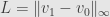 be exactly the supremum norm of the difference between the first two functions in the sequence. I say that
  . Indeed, we calculate inductively

Now we can bound the distance between any two functions in the sequence. If  are two indices we calculate:
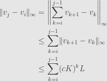
But this is a chunk of a geometric series; since , the series must converge, and so we can make this sum as small as we please by choosing and  large enough.
This then tells us that our sequence of functions is  -Cauchy, and thus -convergent, which implies uniform pointwise convergence. The uniformity is important because it means that we can exchange integration with the limiting process. That is,

And so we can start with our definition:

and take the limit of both sides
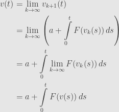
where we have used the continuity of . This shows that the limiting function does indeed satisfy the integral equation, and thus the original initial value problem.
May 6, 2011
Posted by John Armstrong |
Analysis, Differential Equations |
1 Comment
Now we can start actually closing in on a solution to our initial value problem. Recall the setup:
The first thing we’ll do is translate this into an integral equation. Integrating both sides of the first equation and using the second equation we find

Conversely, if satisfies this equation then clearly it satisfies the two conditions in our initial value problem.
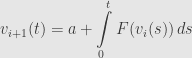
Now the nice thing about this formulation is that it expresses as the fixed point of a certain operation. To find it, we will use an iterative method. We start with  and define the “Picard iteration”
This is sort of like Newton’s method, where we express the point we’re looking for as the fixed point of a function, and then find the fixed point by iterating that very function.
The one catch is, how are we sure that this is well-defined? What could go wrong? Well, how do we know that  is in the domain of ? We have to make some choices to make sure this works out.
First, let be the closed ball of radius  centered on . We pick so that satisfies a Lipschitz condition on , which we know we can do because is locally Lipschitz. Since this is a closed ball and is continuous, we can find an upper bound
  for
for  . Finally, we can find a
  , and the interval . I assert that
  is well-defined.
First of all,  for all , so that’s good. We now assume that is well-defined and prove that
  is as well. It’s clearly well-defined as a function, since
  by assumption, and is contained within the domain of . The integral makes sense since the integrand is continuous, and then we can add . But is
  ?
?
So we calculate

which shows that the difference between  and has length smaller than for any . Thus
  , as asserted, and the Picard iteration is well-defined.
May 5, 2011
Posted by John Armstrong |
Analysis, Differential Equations |
4 Comments
It turns out that our existence proof will actually hinge on our function satisfying a Lipschitz condition. So let’s show that we will have this property anyway.
More specifically, we are given a function  defined on an open region
  . We want to show that around any point
  we have some neighborhood
  where
where  satisfies a Lipschitz condition. That is: for and in the neighborhood , there is a constant and we have the inequality

We don’t have to use the same for each neighborhood, but every point should have a neighborhood with some .
Infinitesimally, this is obvious. The differential  is a linear transformation. Since it goes between finite-dimensional vector spaces it’s bounded, which means we have an inequality
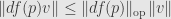
where  is the operator norm of
  . What this lemma says is that if the function is we can make this work out over finite distances, not just for infinitesimal displacements.
So, given our point  let
let  be the closed ball of radius
  around , and choose so small that is contained within . Since the function — which takes points to the space of linear operators — is continuous by our assumption, the function
  is continuous as well. The extreme value theorem tells us that since is compact this continuous function must attain a maximum, which we call .
The ball is also “convex”, meaning that given points and in the ball the whole segment  for
for  is contained within the ball. We define a function
  and use the chain rule to calculate

Then we calculate

And from this we conclude
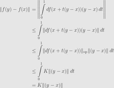
That is, the separation between the outputs is expressible as an integral, the integrand of which is bounded by our infinitesimal result above. Integrating up we get the bound we seek.
May 4, 2011
Posted by John Armstrong |
Analysis, Differential Equations |
3 Comments
I have to take a little detour for now to prove an important result: the existence and uniqueness theorem of ordinary differential equations. This is one of those hard analytic nubs that differential geometry takes as a building block, but it still needs to be proven once before we can get back away from this analysis.
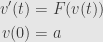
Anyway, we consider a continuously differentiable function  defined on an open region , and the initial value problem:
for some fixed initial value . I say that there is a unique solution to this problem, in the sense that there is some interval  and a unique function
  satisfying both conditions.
In fact, more is true: the solution varies continuously with the starting point. That is, there is an interval  around , some neighborhood
  of and a continuously differentiable function
  called the “flow” of the system defined by the differential equation
  , which satisfies the two conditions:

Then for any  we can get a curve
  defined by
  . The two conditions on the flow then tell us that
  is a solution of the initial value problem with initial value
  .
.
This will take us a short while, but then we can put it behind us and get back to differential geometry. Incidentally, the approach I will use generally follows that of Hirsch and Smale.
May 4, 2011
Posted by John Armstrong |
Analysis, Differential Equations |
4 Comments