I just spent all day on the road back to NOLA to handle some end-of-month business, clean out my office, and so on. This one will have to do for today and tomorrow.
It gets annoying to write out matrices using the embedded LaTeX here, but I suppose I really should, just for thoroughness’ sake.
In general, a matrix is a collection of field elements with an upper and a lower index. We can write out all these elements in a rectangular array. The upper index should list the rows of our array, while the lower index should list the columns. The matrix  with entries
  for
for  running from
  to
to  and
and  running from to is written out in full as
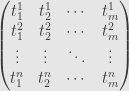
We call this an  matrix, because the array is rows high and columns wide.
There is a natural isomorphism 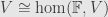 . This means that every vector in dimension , written out in the components relative to a given basis, can be seen as an
  “column vector”:

Similarly, a linear functional on an -dimensional space can be written as a  “row vector”:

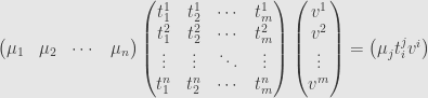
Notice that evaluation of linear transformations is now just a special case of matrix multiplication! Let’s practice by writing out the composition of a linear functional  , a linear map
  , and a vector
  .
.

A matrix product makes sense if and only if the number of columns in the left-hand matrix is the same as the number of rows in the right-hand matrix. That is, an  and an
  can be multiplied. The result will be an
  matrix. We calculate it by taking a row from the left-hand matrix and a column from the right-hand matrix. Since these are the same length (by assumption) we can multiply corresponding elements and sum up.
In the example above, the matrix and the matrix  can be multiplied. There is only one column in the latter to pick, so we simply choose row
  out of on the left:
  . Multiplying corresponding elements and summing gives the single field element
  (remember the summation convention). We get of these elements — one for each row — and we arrange them in a new
  matrix:

Then we can multiply the row vector  by this column vector to get the
  matrix:
Just like we slip back and forth between vectors and matrices, we will usually consider a field element and the matrix with that single entry as being pretty much the same thing.
The first multiplication here turned an -dimensional (column) vector into an -dimensional one, reflecting the source and target of the transformation  . Then we evaluated the linear functional
  on the resulting vector. But by the associativity of matrix multiplication we could have first multiplied on the left:

turning the linear functional on  into one on
  . But this is just the dual transformation
  ! Then we can evaluate this on the column vector to get the same result:
  .
.
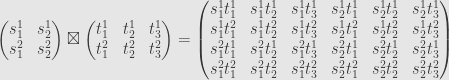
There is one slightly touchy thing we need to be careful about: Kronecker products. When the upper index is a pair  with
with  and
and  we have to pick an order on the set of such pairs. We’ll always use the “lexicographic” order. That is, we start with
  , then
  , and so on until
  before starting over with
  ,
,  , and so on. Let’s write out a couple examples just to be clear:

So the Kronecker product depends on the order of multiplication. But this dependence is somewhat illusory. The only real difference is reordering the bases we use for the tensor products of the vector spaces involved, and so a change of basis can turn one into the other. This is an example of how matrices can carry artifacts of our choice of bases.
May 30, 2008
Posted by John Armstrong |
Algebra, Linear Algebra |
7 Comments
Like we saw with the tensor product of vector spaces, the dual space construction turns out to be a functor. In fact, it’s a contravariant functor. That is, if we have a linear transformation  we get a linear transformation
  . As usual, we ask what this looks like for matrices.
First, how do we define the dual transformation? It turns out this is the contravariant functor represented by  . That is, if
  is a linear functional, we define
  . In terms of the action on vectors,
 =\mu(T(v))](https://s0.wp.com/latex.php?latex=%5Cleft%5BT%5E%2A%28%5Cmu%29%5Cright%5D%28v%29%3D%5Cmu%28T%28v%29%29&bg=e6e6e6&fg=333333&s=0&c=20201002)
Now let’s assume that  and
and  are finite-dimensional, and pick bases
  and
and  for and , respectively. Then the linear transformation has matrix coefficients
  . We also get the dual bases
  of
of  and
and  of
of  .
.
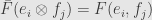
Given a basic linear functional  on , we want to write
  in terms of the
  . So let’s evaluate it on a generic basis vector
  and see what we get. The formula above shows us that
=\phi^l(T(e_i))=\phi^l(t_i^kf_k)=t_i^k\delta_k^l=t_i^l](https://s0.wp.com/latex.php?latex=%5Cleft%5BT%5E%2A%28%5Cphi%5El%29%5Cright%5D%28e_i%29%3D%5Cphi%5El%28T%28e_i%29%29%3D%5Cphi%5El%28t_i%5Ekf_k%29%3Dt_i%5Ek%5Cdelta_k%5El%3Dt_i%5El&bg=e6e6e6&fg=333333&s=0&c=20201002)
In other words, we can write  . The same matrix works, but we use its indices differently.
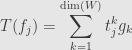
In general, given a linear functional with coefficients  we find the coefficients of
  as
as  . The value
 =\mu(T(u))](https://s0.wp.com/latex.php?latex=%5Cleft%5BT%5E%2A%28%5Cmu%29%5Cright%5D%28v%29%3D%5Cmu%28T%28u%29%29&bg=e6e6e6&fg=333333&s=0&c=20201002) becomes
becomes  . Notice that the summation convention tells us this must be a scalar (as we expect) because there are no unpaired indices. Also notice that because we can use the same matrix for two different transformations we seem to have an ambiguity: is the lower index running over a basis for or one for ? Luckily, since every basis gives rise to a dual basis, we don’t need to care. Both spaces have the same dimension anyhow.
May 28, 2008
Posted by John Armstrong |
Algebra, Linear Algebra |
2 Comments
Another thing vector spaces come with is duals. That is, given a vector space we have the dual vector space  of “linear functionals” on — linear functions from to the base field . Again we ask how this looks in terms of bases.
So let’s take a finite-dimensional vector space with basis , and consider some linear functional  . Like any linear function, we can write down matrix coefficients
  . Notice that since our target space (the base field ) is only one-dimensional, we don’t need another index to count its basis.
Now let’s consider a specially-crafted linear functional. We can define one however we like on the basis vectors and then let linearity handle the rest. So let’s say our functional takes the value on  and the value
  on every other basis element. We’ll call this linear functional
  . Notice that on any vector we have

so it returns the coefficient of . There’s nothing special about here, though. We can define functionals by setting  . This is the “Kronecker delta”, and it has the value when its two indices match, and when they don’t.
Now given a linear functional with matrix coefficients  , let’s write out a new linear functional
  . What does this do to basis elements?

so this new transformation has exactly the same matrix as does. It must be the same transformation! So any linear functional can be written uniquely as a linear combination of the , and thus they form a basis for the dual space. We call the “dual basis” to .
Now if we take a generic linear functional and evaluate it on a generic vector  we find

Once we pick a basis for we immediately get a basis for , and evaluation of a linear functional on a vector looks neat in terms of these bases.
May 27, 2008
Posted by John Armstrong |
Algebra, Linear Algebra |
30 Comments
Given two finite-dimensional vector spaces and , with bases and  respectively, we know how to build a tensor product: use the basis
  .
.
But an important thing about the tensor product is that it’s a functor. That is, if we have linear transformations  and
and  , then we get a linear transformation
  . So what does this operation look like in terms of matrices?
First we have to remember exactly how we get the tensor product  . Clearly we can consider the function
  . Then we can compose with the bilinear function
  to get a bilinear function from
  to
to  . By the universal property, this must factor uniquely through a linear function
  . It is this map we call .
We have to pick bases  of
of  and
and  of
of  . This gives us a matrix coefficients
  for
for  and
and  for . To calculate the matrix for we have to evaluate it on the basis elements
  of
of  . By definition we find:
=S(e_i)\otimes T(f_j)=\left(s_i^ke_k'\right)\otimes\left(t_j^lf_l'\right)=s_i^kt_j^le_k'\otimes f_l'](https://s0.wp.com/latex.php?latex=%5Cleft%5BS%5Cotimes+T%5Cright%5D%28e_i%5Cotimes+f_j%29%3DS%28e_i%29%5Cotimes+T%28f_j%29%3D%5Cleft%28s_i%5Eke_k%27%5Cright%29%5Cotimes%5Cleft%28t_j%5Elf_l%27%5Cright%29%3Ds_i%5Ekt_j%5Ele_k%27%5Cotimes+f_l%27&bg=e6e6e6&fg=333333&s=0&c=20201002)
that is, the matrix coefficient between the index pair  and the index pair
  is
is  .
.
It’s not often taught anymore, but there is a name for this operation: the Kronecker product. If we write the matrices (as opposed to just their coefficients)  and
and  , then we write the Kronecker product
  .
.
May 26, 2008
Posted by John Armstrong |
Algebra, Linear Algebra |
6 Comments
Since we’re looking at vector spaces, which are special kinds of modules, we know that  has a tensor product structure. Let’s see what this means when we pick bases.
First off, let’s remember what the tensor product of two vector spaces and is. It’s a new vector space and a bilinear (linear in each of two variables separately) function  satisfying a certain universal property. Specifically, if
  is any bilinear function it must factor uniquely through
  as
as  . The catch here is that when we say “linear” and “bilinear” we mean that the functions preserve both addition and scalar multiplication. As with any other universal property, such a tensor product will be uniquely defined up to isomorphism.
So let’s take finite-dimensional vector spaces and , and bases of and of . I say that the vector space with basis , and with the bilinear function 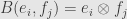 is a tensor product. Here the expression is just a name for a basis element of the new vector space. Such elements are indexed by the set of pairs , where indexes a basis for and indexes a basis for .
First off, what do I mean by the bilinear function ? Just as for linear functions, we can define bilinear functions by defining them on bases. That is, if we have  and
and  , we get the vector

in our new vector space, with coefficients  .
.
So let’s take a bilinear function  and define a linear function
  by setting
We can easily check that does indeed factor as desired, since

so on basis elements. By linearity, they must agree for all pairs  . It should also be clear that we can’t define any other way and hope to satisfy this equation, so the factorization is unique.
Thus if we have bases of and of , we immediately get a basis of . As a side note, we immediately see that the dimension of the tensor product of two vector spaces is the product of their dimensions.
May 23, 2008
Posted by John Armstrong |
Algebra, Linear Algebra |
5 Comments
With the summation convention firmly in hand, we continue our discussion of matrices.
We’ve said before that the category of vector space is enriched over itself. That is, if we have vector spaces and over the field , the set of linear transformations  is itself a vector space over . In fact, it inherits this structure from the one on . We define the sum and the scalar product
=S(u)+T(u)](https://s0.wp.com/latex.php?latex=%5Cleft%5BS%2BT%5Cright%5D%28u%29%3DS%28u%29%2BT%28u%29&bg=e6e6e6&fg=333333&s=0&c=20201002)
=cT(u)](https://s0.wp.com/latex.php?latex=%5Cleft%5BcT%5Cright%5D%28u%29%3DcT%28u%29&bg=e6e6e6&fg=333333&s=0&c=20201002)
for linear transformations and from to , and for a constant  . Verifying that these are also linear transformations is straightforward.
So what do these structures look like in the language of matrices? If and are finite-dimensional, let’s pick bases of and of . Now we get matrix coefficients  and , where indexes the basis of and indexes the basis of . Now we can calculate the matrices of the sum and scalar product above.
We do this, as usual, by calculating the value the transformations take at each basis element. First, the sum:
=S(e_i)+T(e_i)=s_i^jf_j+t_i^jf_j=(s_i^j+t_i^j)f_j](https://s0.wp.com/latex.php?latex=%5Cleft%5BS%2BT%5Cright%5D%28e_i%29%3DS%28e_i%29%2BT%28e_i%29%3Ds_i%5Ejf_j%2Bt_i%5Ejf_j%3D%28s_i%5Ej%2Bt_i%5Ej%29f_j&bg=e6e6e6&fg=333333&s=0&c=20201002)
and now the scalar product:
=cT(e_i)=(ct_i^j)f_j](https://s0.wp.com/latex.php?latex=%5Cleft%5BcT%5Cright%5D%28e_i%29%3DcT%28e_i%29%3D%28ct_i%5Ej%29f_j&bg=e6e6e6&fg=333333&s=0&c=20201002)
so we calculate the matrix coefficients of the sum of two linear transformations by adding the corresponding matrix coefficients of each transformation, and the matrix coefficients of the scalar product by multiplying each coefficient by the same scalar.
May 22, 2008
Posted by John Armstrong |
Algebra, Linear Algebra |
1 Comment
Look at the formulas we were using yesterday. There’s a lot of summations in there, and a lot of big sigmas. Those get really tiring to write over and over, and they get tiring really quick. Back when Einstein was writing up his papers, he used a lot of linear transformations, and wrote them all out in matrices. Accordingly, he used a lot of those big sigmas.
When we’re typing nowadays, or when we write on a pad or on the board, this isn’t a problem. But remember that up until very recently, publications had to actually set type. Actual little pieces of metal with characters raised (and reversed!) on them would get slathered with ink and pressed to paper. Incidentally, this is why companies that produce fonts are called “type foundries”. They actually forged those metal bits with letter shapes in different styles, and sold sets of them to printers.
Now Einstein was using a lot of these big sigmas, and there were pages that had so many of them that the printer would run out! Even if they set one page at once and printed them off, they just didn’t have enough little pieces of metal with big sigmas on them to handle it. Clearly something needed to be done to cut down on demand for them.
Here we note that we’re always summing over some basis. Even if there’s no basis element in a formula — say, the formula for a matrix product — the summation is over the dimension of some vector space. We also notice that when we chose to write some of our indices as subscripts and some as superscripts, we’re always summing over one of each. We now adopt the convention that if we ever see a repeated index — once as a superscript and once as a subscript — we’ll read that as summing over an appropriate basis.
For example, when we wanted to write a vector  , we had to take the basis
  of and write up the sum

but now we just write  . The repeated index and the fact that we’re talking about a vector in means we sum for running from to the dimension of . Similarly we write out the value of a linear transformation on a basis vector:
  . Here we determine from context that
  should run from to the dimension of
  .
.
What about finding the coefficients of a linear transformation acting on a vector? Before we wrote this as

Where now we write the result as  . Since the
  are the coefficients of a vector in , must run from to the dimension of .
And similarly given linear transformations  and
and  represented (given choices of bases) by the matrices with components and
  , the matrix of their product is then written
  . Again, we determine from context that we should be summing over a set indexing a basis for .
One very important thing to note here is that it’s not going to matter what basis for we use here! I’m not going to prove this quite yet, but built right into this notation is the fact that the composite of the two transformations is completely independent of the choice of basis of . Of course, the matrix of the composite still depends on the bases of and we pick, but the dependence on vanishes as we take the sum.
Einstein had a slightly easier time of things: he was always dealing with four-dimensional vector spaces, so all his indices had the same range of summation. We’ve got to pay some attention here and be careful about what vector space a given index is talking about, but in the long run it saves a lot of time.
May 21, 2008
Posted by John Armstrong |
Fundamentals, Linear Algebra |
18 Comments
Yesterday we talked about the high-level views of linear algebra. That is, we’re discussing the category of vector spaces over a field and -linear transformations between them.
More concretely, now: we know that every vector space over is free as a module over . That is, every vector space has a basis — a set of vectors so that every other vector can be uniquely written as an -linear combination of them — though a basis is far from unique. Just how nonunique it is will be one of our subjects going forward.
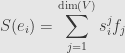
Now if we’ve got a linear transformation from one finite-dimensional vector space to another, and if we have a basis  of and a basis
  of , we can use these to write the transformation in a particular form: as a matrix. Take the transformation and apply it to each basis element of to get vectors
  . These can be written uniquely as linear combinations
for certain  . These coefficients, collected together, we call a matrix. They’re enough to calculate the value of the transformation on any vector , because we can write

We’re writing the indices of the components as superscripts here, just go with it. Then we can evaluate  using linearity
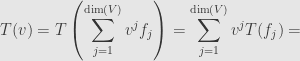

So the coefficients defining the vector and the matrix coefficients together give us the coefficients defining the vector  .
.
If we have another finite-dimensional vector space with basis  and another transformation then we have another matrix
Now we can compose these two transformations and calculate the result on a basis element
=T\left(S(e_i)\right)=T\left(\sum_{j=1}^{\mathrm{dim}(V)}s_i^jf_j\right)=\sum_{j=1}^{\mathrm{dim}(V)}s_i^jT(f_j)=](https://s0.wp.com/latex.php?latex=%5Cdisplaystyle+%5Cleft%5BT%5Ccirc+S%5Cright%5D%28e_i%29%3DT%5Cleft%28S%28e_i%29%5Cright%29%3DT%5Cleft%28%5Csum_%7Bj%3D1%7D%5E%7B%5Cmathrm%7Bdim%7D%28V%29%7Ds_i%5Ejf_j%5Cright%29%3D%5Csum_%7Bj%3D1%7D%5E%7B%5Cmathrm%7Bdim%7D%28V%29%7Ds_i%5EjT%28f_j%29%3D&bg=e6e6e6&fg=333333&s=0&c=20201002)

This last quantity in parens is then the matrix of the composite transformation  . Thus we can represent the operation of composition by this formula for matrix multiplication.
May 20, 2008
Posted by John Armstrong |
Algebra, Linear Algebra |
7 Comments
Here we begin a discussion of linear algebra. There are three views on what this is all about.
The mid-level view is that we’re studying the properties of linear maps — homomorphisms — between abelian groups, and particularly between modules or vector spaces, which are just modules over a field. In particular we’ll focus on vector spaces over some arbitrary (but fixed!) field .
The high-level view is that what we’re really studying is the category of -modules. Categories are all about how morphisms between their objects interact, so this is what we’re really after here. And it turns out we already know a lot about these sorts of categories! Specifically, they’re abelian categories. In fact, since we’re working over a field (which is a commutative ring) the properties of  -functors tell us that
  is enriched over itself.
So this tells us that our category of vector spaces has a biproduct — the direct sum — and in particular a zero object — the trivial -dimensional vector space  . It also has a tensor product, which makes this a monoidal category, using the one-dimensional vector space itself as monoidal identity. We also know that kernels and cokernels exist, which then (along with biproducts) give us all finite limits and colimits.
The third viewpoint is that we’re talking about solving systems of linear equations, and that’s where “linear algebra” comes from. The connection between these abstract formulations and that concrete one is a bit mysterious at first blush, but we’ll start making it tomorrow.
May 19, 2008
Posted by John Armstrong |
Algebra, Linear Algebra |
4 Comments
Okay, here’s the part I promised I’d finish last Friday. How do we deal with rearrangements that “go to infinity” more than once? That is, we chop up the infinite set of natural numbers into a bunch of other infinite sets, add each of these subseries up, and then add the results up. If the original series was absolutely convergent, we’ll get the same answer.
First of all, if a series  converges absolutely, then so does any subseries
  , where
  is an injective (but not necessarily bijective!) function from the natural numbers to themselves. For instance, we could let
  and add up all the even terms from the original series.
To see this, notice that at any finite we have a maximum value 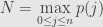 . Then we find

So the new sequence of partial sums of absolute values is increasing and bounded above, and thus converges.
Now let’s let  ,
,  ,
,  , and so on be a countable collection of functions defined on the natural numbers. We ask that
- Each
 is injective.
- The image of is a subset
 .
.
- The collection
 is a partition of
  . That is, these subsets are mutually disjoint, and their union is all of .
If is an absolutely convergent series, we define  — the subseries defined by . Then from what we said above, each
  is an absolutely convergent series whose sum we call
  . We assert now that
  is an absolutely convergent series whose sum is the same as that of .
Let’s set  . That is, we have

But this is just the sum of a bunch of absolute values from the original series, and so is bounded by  . So the series of absolute values of has bounded partial sums, and so converges absolutely. That it has the same sum as the original is another argument exactly analogous to (but more complicated than) the one for a simple rearrangement, and for associativity of absolutely convergent series.
This pretty much wraps up all I want to say about calculus for now. I’m going to take a little time to regroup before I dive into linear algebra in more detail than the abstract algebra I covered before. But if you want to get ahead, go back and look over what I said about rings and modules. A lot of that will be revisited and fleshed out in the next sections.
May 12, 2008
Posted by John Armstrong |
Analysis, Calculus |
3 Comments

