The Implicit Function Theorem I

Let’s consider the function $F(x,y)=x^2+y^2-1$ . The collection of points $(x,y)$ so that $F(x,y)=0$ defines a curve in the plane: the unit circle. Unfortunately, this relation is not a function. Neither is $y$ defined as a function of $x$ , nor is $x$ defined as a function of $y$ by this curve. However, if we consider a point $(a,b)$ on the curve (that is, with $F(a,b)=0$ ), then near this point we usually do have a graph of $x$ as a function of $y$ (except for a few isolated points). That is, as we move $y$ near the value $b$ then we have to adjust $x$ to maintain the relation $F(x,y)=0$ . There is some function $f(y)$ defined “implicitly” in a neighborhood of $b$ satisfying the relation $F(f(y),y)=0$ .

We want to generalize this situation. Given a system of $n$ functions of $n+m$ variables

$\displaystyle f^i(x;t)=f^i(x^1,\dots,x^n;t^1,\dots,t^m)$

we consider the collection of points $(x;t)$ in $n+m$ -dimensional space satisfying $f(x;t)=0$ .

If this were a linear system, the rank-nullity theorem would tell us that our solution space is (generically) $m$ dimensional. Indeed, we could use Gauss-Jordan elimination to put the system into reduced row echelon form, and (usually) find the resulting matrix starting with an $n\times n$ identity matrix, like

$\displaystyle\begin{pmatrix}1&0&0&2&1\\{0}&1&0&3&0\\{0}&0&1&-1&1\end{pmatrix}$

This makes finding solutions to the system easy. We put our $n+m$ variables into a column vector and write

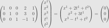
$\displaystyle\begin{pmatrix}1&0&0&2&1\\{0}&1&0&3&0\\{0}&0&1&-1&1\end{pmatrix}\begin{pmatrix}x^1\\x^2\\x^3\\t^1\\t^2\end{pmatrix}=\begin{pmatrix}x^1+2t^1+t^2\\x^2+3t^1\\x^3-t^1+t^2\end{pmatrix}=\begin{pmatrix}0\\{0}\\{0}\end{pmatrix}$

and from this we find

$\displaystyle\begin{aligned}x^1&=-2t^1-t^2\\x^2&=-3t^1\\x^3&=t^1-t^2\end{aligned}$

Thus we can use the $m$ variables $t^j$ as parameters on the space of solutions, and define each of the $x^i$ as a function of the $t^j$ .

But in general we don’t have a linear system. Still, we want to know some circumstances under which we can do something similar and write each of the $x^i$ as a function of the other variables $t^j$ , at least near some known point $(a;b)$ .

The key observation is that we can perform the Gauss-Jordan elimination above and get a matrix with rank $n$ if and only if the leading $n\times n$ matrix is invertible. And this is generalized to asking that some Jacobian determinant of our system of functions is nonzero.

Specifically, let’s assume that all of the $f^i$ are continuously differentiable on some region $S$ in $n+m$ -dimensional space, and that $(a;b)$ is some point in $S$ where $f(a;b)=0$ , and at which the determinant

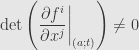
$\displaystyle\det\left(\frac{\partial f^i}{\partial x^j}\bigg\vert_{(a;t)}\right)\neq0$

where both indices $i$ and $j$ run from $1$ to $n$ to make a square matrix. Then I assert that there is some $k$ -dimensional neighborhood $T$ of $b$ and a uniquely defined, continuously differentiable, vector-valued function $g:T\rightarrow\mathbb{R}^n$ so that $g(b)=a$ and $f(g(t);t)=0$ .

That is, near $(a;b)$ we can use the variables $t^j$ as parameters on the space of solutions to our system of equations. Near this point, the solution set looks like the graph of the function $x=g(t)$ , which is implicitly defined by the need to stay on the solution set as we vary $t$ . This is the implicit function theorem, and we will prove it next time.

November 19, 2009 - Posted by John Armstrong | Analysis, Calculus

4 Comments »

[…] Implicit Function Theorem II Okay, today we’re going to prove the implicit function theorem. We’re going to think of our function as taking an -dimensional vector and a -dimensional […]

Pingback by The Implicit Function Theorem II « The Unapologetic Mathematician | November 20, 2009 | Reply
[…] extremely difficult. At least we do know that such a parameterization will often exist. Indeed, the implicit function theorem tells us that if we have continuously differentiable constraint functions whose zeroes describe a […]

Pingback by Extrema with Constraints I « The Unapologetic Mathematician | November 25, 2009 | Reply
[…] this, we’ll write , so we can write the point as and particularly . Now we can invoke the implicit function theorem! We find an -dimensional neighborhood of and a unique continuously differentiable function so […]

Pingback by Extrema with Constraints II « The Unapologetic Mathematician | November 27, 2009 | Reply
[…] can also recall the implicit function theorem. This is less directly generalizable to manifolds, since talking about a function is effectively […]

Pingback by The Implicit Function Theorem « The Unapologetic Mathematician | April 15, 2011 | Reply

About this weblog

This is mainly an expository blath, with occasional high-level excursions, humorous observations, rants, and musings. The main-line exposition should be accessible to the “Generally Interested Lay Audience”, as long as you trace the links back towards the basics. Check the sidebar for specific topics (under “Categories”).

I’m in the process of tweaking some aspects of the site to make it easier to refer back to older topics, so try to make the best of it for now.

RSS Feeds

RSS - Posts
RSS - Comments
Feedback

Got something to say? Anonymous questions, comments, and suggestions at Formspring.me!
Subjects

Subjects
Archives

November 2009

M T W T F S S

1

2 3 4 5 6 7 8

9 10 11 12 13 14 15

16 17 18 19 20 21 22

23 24 25 26 27 28 29

30

« Oct Dec »
Search for:

The Unapologetic Mathematician

Mathematics for the interested outsider