The flip side of the line integral is the surface integral.
Given an  -manifold
  we let
  be an oriented
  -dimensional “hypersurface”, which term we use because in the usual case of
  a hypersurface has two dimensions — it’s a regular surface. The orientation on a hypersurface consists of tangent vectors which are all in the image of the derivative of the local parameterization map, which is a singular cube.
Now we want another way of viewing this orientation. Given a metric on we can use the inverse of the Hodge star from on the orientation -form of , which gives us a covector  defined at each point
  of . Roughly speaking, the orientation form of defines an -dimensional subspace of
  : the covectors “tangent to “. The covector
  is “perpendicular to
  , and since has only one fewer dimension than there are only two choices for the direction of such a vector. The choice of one or the other defines a distinction between the two sides of .
If we flip around our covectors into vectors — again using the metric — we get something like a vector field defined on . I say “something like” because it’s only defined on , which is not an open subspace of , and strictly speaking a vector field must be defined on an open subspace. It’s not hard to see that we could “thicken up” into an open subspace and extend our vector field smoothly there, so I’m not really going to make a big deal of it, but I want to be careful with my language; it’s also why I didn’t say we get a  -form from the Hodge star. Anyway, we will call this vector-valued function
  , for reasons that will become apparent shortly.
Now what if we have another vector-valued function  defined on — for example, it could be a vector field defined on an open subspace containing . We can define the “surface integral of through “, which measures how much the vector field flows through the surface in the direction our orientation picks out as “positive”. And we measure this amount at any given point by taking the covector at provided by the Hodge star and evaluating it at the vector
  . This gives us a value that we can integrate over the surface. This evaluation can be flipped around into our vector field notation and language, allowing us to write down the integral as

because the “dot product” ](https://s0.wp.com/latex.php?latex=%5Cleft%5BF%5Ccdot+dS%5Cright%5D%28p%29&bg=e6e6e6&fg=333333&s=0&c=20201002) is exactly what it means to evaluate the covector dual to
is exactly what it means to evaluate the covector dual to  at the vector . This should look familiar from multivariable calculus, but I’ve been saying that a lot lately, haven’t I?
We can also go the other direction and make things look more abstract. We could write our vector field as a -form  , which lets us write our surface integral as
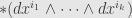
where  is the volume form on . But then we know that
  the volume form on . That is, we can define a hypersurface integral of any -form across any hypersurface equipped with a volume form
  by
by

whether or not we have a metric on .
October 27, 2011
Posted by John Armstrong |
Differential Geometry, Geometry |
3 Comments
At last we can state one of our special cases of Stokes’ theorem. We don’t need to prove it, since we already did in far more generality, but it should help put our feet on some familiar ground.
So, we take an oriented curve  in a manifold . The image of is an oriented submanifold of , where the “orientation” means picking one of the two possible tangent directions at each point along the image of the curve. As a high-level view, we can characterize the orientation as the direction that we traverse the curve, from one “starting” endpoint to the other “ending” endpoint.
Given any -form on the image of — in particular, given an defined on — we can define the line integral of over . We already have a way of evaluating line integrals: pull the -form back to the parameter interval of and integrate there as usual. But now we want to use Stokes’ theorem to come up with another way. Let’s write down what it will look like:

where  is some
  -form. That is: a function. This tells us that we can only make this work for “exact” -forms , which can be written in the form
  for some function
  .
.
But if this is the case, then life is beautiful. The (oriented) boundary of is easy: it consists of two -faces corresponding to the two endpoints. The starting point gets a negative orientation while the ending point gets a positive orientation. And so we write

That is, we just evaluate at the two endpoints and subtract the value at the start from the value at the end!
What does this look like when we have a metric and we can rewrite the -form as a vector field ? In this case, is exact if and only if is “conservative”, which just means that  for some function . Then we can write

which should look very familiar from multivariable calculus.
We call this the fundamental theorem of line integrals by analogy with the fundamental theorem of calculus. Indeed, if we set this up in the manifold  , we get back exactly the second part of the fundamental theorem of calculus back again.
October 24, 2011
Posted by John Armstrong |
Differential Geometry, Geometry |
6 Comments
We now define some particular kinds of integrals as special cases of our theory of integrals over manifolds. And the first such special case is that of a line integral.
Consider an oriented curve in the manifold . We know that this is a singular -cube, and so we can pair it off with a -form . Specifically, we pull back to  on the interval
 ![[0,1]](https://s0.wp.com/latex.php?latex=%5B0%2C1%5D&bg=e6e6e6&fg=333333&s=0&c=20201002) and integrate.
and integrate.
More explicitly, the pullback is evaluated as
=\left[\alpha_{c(t_0)}\right]\left(c_{*t_0}\frac{d}{dt}\bigg\vert_{t_0}\right)](https://s0.wp.com/latex.php?latex=%5Cdisplaystyle%5Cleft%5Bc%5E%2A%5Calpha%5Cleft%28%5Cfrac%7Bd%7D%7Bdt%7D%5Cright%29%5Cright%5D%28t_0%29%3D%5Cleft%5B%5Calpha_%7Bc%28t_0%29%7D%5Cright%5D%5Cleft%28c_%7B%2At_0%7D%5Cfrac%7Bd%7D%7Bdt%7D%5Cbigg%5Cvert_%7Bt_0%7D%5Cright%29&bg=e6e6e6&fg=333333&s=0&c=20201002)
That is, for a ![t_0\in[0,1]](https://s0.wp.com/latex.php?latex=t_0%5Cin%5B0%2C1%5D&bg=e6e6e6&fg=333333&s=0&c=20201002) , we take the value
, we take the value  of the -form at the point
  and the tangent vector
  and pair them off. This gives us a real-valued function which we can integrate over the interval.
So, why do we care about this particularly? In the presence of a metric, we have an equivalence between -forms and vector fields . And specifically we know that the pairing  is equal to the inner product
  — this is how the equivalence is defined, after all. And thus the line integral looks like
![\displaystyle\int\limits_c\alpha=\int\limits_{[0,1]}\langle F(c(t)),c'(t)\rangle\,dt](https://s0.wp.com/latex.php?latex=%5Cdisplaystyle%5Cint%5Climits_c%5Calpha%3D%5Cint%5Climits_%7B%5B0%2C1%5D%7D%5Clangle+F%28c%28t%29%29%2Cc%27%28t%29%5Crangle%5C%2Cdt&bg=e6e6e6&fg=333333&s=0&c=20201002)
Often the inner product is written with a dot — usually called the “dot product” of vectors — in which case this takes the form
![\displaystyle\int\limits_{[0,1]}F(c(t))\cdot c'(t)\,dt](https://s0.wp.com/latex.php?latex=%5Cdisplaystyle%5Cint%5Climits_%7B%5B0%2C1%5D%7DF%28c%28t%29%29%5Ccdot+c%27%28t%29%5C%2Cdt&bg=e6e6e6&fg=333333&s=0&c=20201002)
We also often write  as a “vector differential-valued function”, in which case we can write
![\displaystyle\int\limits_{[0,1]}F\cdot ds](https://s0.wp.com/latex.php?latex=%5Cdisplaystyle%5Cint%5Climits_%7B%5B0%2C1%5D%7DF%5Ccdot+ds&bg=e6e6e6&fg=333333&s=0&c=20201002)
Of course, we often parameterize a curve by a more general interval  than , in which case we write

This expression may look familiar from multivariable calculus, where we first defined line integrals. We can now see how this definition is a special case of a much more general construction.
October 21, 2011
Posted by John Armstrong |
Differential Geometry, Geometry |
5 Comments
From our calculation of the square of the Hodge star we can tell that the star operation is invertible. Indeed, since  — applying the star twice to a
  -form in an -manifold with metric
  is the same as multiplying it by
  and the determinant of the matrix of — we conclude that
  .
.
With this inverse in hand, we will define the “codifferential”

The first star sends a -form to an  -form; the exterior derivative sends it to an
  -form; and the inverse star sends it to a
  -form. Thus the codifferential goes in the opposite direction from the differential — the exterior derivative.
Unfortunately, it’s not quite as algebraically nice. In particular, it’s not a derivation of the algebra. Indeed, we can consider  and
and  in
in  and calculate
while
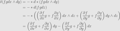
but there is no version of the Leibniz rule that can account for the second and third terms in this latter expansion. Oh well.
On the other hand, the codifferential  is (sort of) the adjoint to the differential. Adjointness would mean that if
  is a -form and
  is a
is a  -form, then
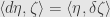
where these inner products are those induced on differential forms from the metric. This doesn’t quite hold, but we can show that it does hold “up to homology”. We can calculate their difference times the canonical volume form
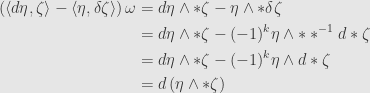
which is an exact -form. It’s not quite as nice as equality, but if we pass to De Rham cohomology it’s just as good.
October 21, 2011
Posted by John Armstrong |
Differential Geometry, Geometry |
Leave a comment
It’s interesting to look at what happens when we apply the Hodge star twice. We just used the fact that in our special case of we always get back exactly what we started with. That is, in this case,  — the identity operation.
It’s easiest to work this out in coordinates. If 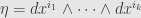 is some -fold wedge then
  is
is  times the wedge of all the indices that don’t show up in . But then
  is times the wedge of all the indices that don’t show up in , which is exactly all the indices that were in in the first place! That is,
 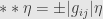 , where the sign is still a bit of a mystery.
But some examples will quickly shed some light on this. We can even extend to the pseudo-Riemannian case and pick a coordinate system so that  , where
  . That is, any two
  are orthogonal, and each either has “squared-length” or
  . The determinant
  is simply the product of all these signs. In the Riemannian case this is simply .
Now, let’s start with an easy example: let be the wedge of the first indices:

Then is (basically) the wedge of the other indices:

The sign is positive since  already has the right order. But now we flip this around the other way:

but this should obey the same rule as ever:

where we pick up a factor of each time we pull one of the last -forms leftwards past the first . We conclude that the actual sign must be  so that this result is exactly . Similar juggling for other selections of will give the same result.
In our special Riemannian case with  , then no matter what is we find the sign is always positive, as we expected. The same holds true in any odd dimension for Riemannian manifolds. In even dimensions, when is odd then so is , and so
  — the negative of the identity transformation. And the whole situation gets more complicated in the pseudo-Riemannian version depending on the number of s in the diagonalized metric tensor.
October 18, 2011
Posted by John Armstrong |
Differential Geometry, Geometry |
5 Comments
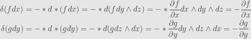
One fact that I didn’t mention when discussing the curl operator is that the curl of a gradient is zero:  . In our terms, this is a simple consequence of the nilpotence of the exterior derivative. Indeed, when we work in terms of -forms instead of vector fields, the composition of the two operators is
  , and
, and  is always zero.
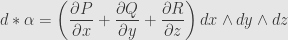
So why do we bring this up now? Because one of the important things to remember from multivariable calculus is that the divergence of a curl is also automatically zero, and this will help us figure out what a divergence is in terms of differential forms. See, if we take our vector field and consider it as a -form, the exterior derivative is already known to be (essentially) the curl. So what else can we do?
We use the Hodge star again to flip the -form back to a  -form, so we can apply the exterior derivative to that. We can check that this will be automatically zero if we start with an image of the curl operator; our earlier calculations show that
  is always the identity mapping — at least on with this metric — so if we first apply the curl
  and then the steps we’ve just suggested, the result is like applying the operator
  .
.
There’s just one catch: as we’ve written it this gives us a  -form, not a function like the divergence operator should! No matter; we can break out the Hodge star once more to flip it back to a -form — a function — just like we want. That is, the divergence operator on -forms is
  .
.
Let’s calculate this in our canonical basis. If we start with a -form  then we first hit it with the Hodge star:

Next comes the exterior derivative:
and then the Hodge star again:

which is exactly the definition (in coordinates) of the usual divergence  of a vector field on .
October 13, 2011
Posted by John Armstrong |
Differential Geometry, Geometry |
3 Comments
Let’s continue our example considering the special case of as an oriented, Riemannian manifold, with the coordinate -forms  forming an oriented, orthonormal basis at each point.
We’ve already see the gradient vector  , which has the same components as the differential
  :
:

This is because we use the metric to convert from vector fields to -forms, and with respect to our usual bases the matrix of the metric is the Kronecker delta.
We will proceed to define analogues of the other classical differential operators you may remember from multivariable calculus. We will actually be defining operators on differential forms, but we will use this same trick to identify vector fields and -forms. We will thus not usually distinguish our operators from the classical ones, but in practice we will use the classical notations when acting on vector fields and our new notations when acting on -forms.
Anyway, the next operator we come to is the curl of a vector field:  . Of course we’ll really start with a -form instead of a vector field, and we already know a differential operator to use on forms. Given a -form we can send it to
  .
.
The only hangup is that this is a -form, while we want the curl of a vector field to be another vector field. But we do have a Hodge star, which we can use to flip a -form back into a -form, which is “really” a vector field again. That is, the curl operator corresponds to the differential operator that takes -forms back to -forms.
Let’s calculate this in our canonical basis, to see that it really does look like the familiar curl. We start with a -form . The first step is to hit it with the exterior derivative, which gives
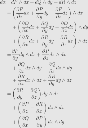
Next we hit this with the Hodge star. We’ve already calculated how the Hodge star affects the canonical basis of -forms, so this is just a simple lookup to find:

which are indeed the usual components of the curl. That is, if is the -form corresponding to the vector field , then  is the -form corresponding to the vector field
  .
.
October 12, 2011
Posted by John Armstrong |
Differential Geometry, Geometry |
8 Comments
I want to start getting into a nice, simple, concrete example of the Hodge star. We need an oriented, Riemannian manifold to work with, and for this example we take , which we cover with the usual coordinate patch with coordinates we call  .
.
To get a metric, we declare the coordinate covector basis  to be orthonormal, which means that we have the matrix
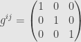
and also the inner product matrix

since we know that  and
and  are inverse matrices. And so we get the canonical volume form

We declare our orientation of to be the one corresponding to this top form.
Okay, so now we can write down the Hodge star in its entirety. And in fact we’ve basically done this way back when we were talking about the Hodge star on a single vector space:

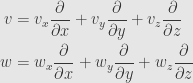
So, what does this buy us? Something else that we’ve seen before in the context of a single vector space. Let’s say that  and
and  are two vector fields defined on an open subset
  . We can write these out in our coordinate basis:
Now, we can use our metric to convert these vectors to covectors — vector fields to -forms. We use the matrix to get

Next we can wedge these together

Now we come to the Hodge star!

and now we’re back to a -form, so we can use the metric to flip it back to a vector field:

Here, the outermost  is the inner product on -forms, while the inner ones are the inner product on vector fields. This is exactly the cross product of vector fields on .
October 11, 2011
Posted by John Armstrong |
Differential Geometry, Geometry |
3 Comments
Let’s say that is an orientable Riemannian manifold. We know that this lets us define a (non-degenerate) inner product on differential forms, and of course we have a wedge product of differential forms. We have almost everything we need to define an analogue of the Hodge star on differential forms; we just need a particular top — or “volume” — form at each point.
To this end, pick one or the other orientation, and let  be a coordinate patch such that the form
  is compatible with the chosen orientation. We’d like to use this form as our top form, but it’s heavily dependent on our choice of coordinates, so it’s very much not a geometric object — our ideal choice of a volume form will be independent of particular coordinates.
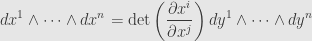
So let’s see how this form changes; if  is another coordinate patch, we can assume that
  by restricting each patch to their common intersection. We’ve already determined that the forms differ by a factor of the Jacobian determinant:
What we want to do is multiply our form by some function that transforms the other way, so that when we put them together the product will be invariant.
Now, we already have something else floating around in our discussion: the metric tensor . When we pick coordinates  we get a matrix-valued function:

and similarly with respect to the alternative coordinates  :
:

So, what’s the difference between these two matrix-valued functions? We can calculate two ways:

That is, we transform the metric tensor with two copies of the inverse Jacobian matrix. Indeed, we could have come up with this on general principles, since has type  — a tensor of type
  transforms with
  copies of the Jacobian and copies of the inverse Jacobian.
Anyway, now we can take the determinant of each side:

and taking square roots we find:

Thus the square root of the metric determinant is a function that transforms from one coordinate patch to the other by the inverse Jacobian determinant. And so we can define:

which does depend on the coordinate system to write down, but which is actually invariant under a change of coordinates! That is,  on the intersection
  . Since the algebras of differential forms form a sheaf
  , we know that we can patch these
  together into a unique
  , and this is our volume form.
And now we can form the Hodge star, point by point. Given any -form we define the dual form to be the unique -form such that

for all -forms  . Since at every point
  we have an inner product and a wedge
  , we can find a
 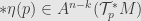 . Some general handwaving will suffice to show that varies smoothly from point to point.
October 6, 2011
Posted by John Armstrong |
Differential Geometry, Geometry |
12 Comments