The Riemann-Stieltjes Integral II

What with cars not working right, I’m not along with the undergraduate math club at the MAA meeting in Lake Charles. That honor goes to Steve Sinnott alone. And so I’m still back in New Orleans, and I may as well write another post today.

Let’s follow on yesterday’s discussion of the Riemann-Stieltjes integral by looking at a restricted sort of integrator. We’ll assume here that is continuously differentiable — that is, that exists and is continuous in the region we care about. We’ll also have a function on hand to integrate.

Now let’s take a tagged partition and set up our Riemann-Stieltjes sum for

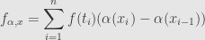
We can also use the partition to set up a Riemann sum for

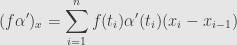
Now the Differential Mean Value Theorem tells us that in each subinterval there is some so that . We stick this into the Riemann-Stieltjes sum and subtract from the Riemann sum

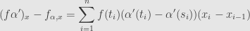
And continuity of tells us that as we pick the partitions finer and finer, we’ll squeeze and together, and so goes to zero. So, when the integrator is continuously differentiable, the Riemann-Stieltjes integral reduces to a Riemann integral

Now let’s go back to the fence story from yesterday. There’s really some function that tells us the height of the fence at position . We got our integrator from the function , which takes a time and gives the position at that time. Thus our function giving height at time is the composition . We also note that as time goes from to , we walk from to . If we put all this into the above equation we find

which is just our change of variables formula.

So here’s what this formula means: we have a real-valued function on some domain — here it’s the height of the fence as a function of position along the ground. We take a region in the space of these variables — the section of the fence we’re walking past — and we “parametrize” it by describing it with a (sufficiently smooth) function taking a single real variable — the position function . We “pull back” our function by composing it with this parametrization, giving us a real-valued function of a real variable, which we can integrate.

The deep thing here is that we have two different parametrizations. We can describe position as meters from a fixed starting point, or we can describe it as the point we’re passing at seconds from a certain starting time. In fact, as we change our function we get all sorts of different parametrizations of the same stretch of ground. And we should measure the same area for the same fence no matter which parametrization we choose.

Given a parametrization , the integral in our recipe will be the Riemann-Stieltjes integral

which we can reduce to the Riemann integral

and it will be the same answer as if we used the “natural” parametrization

And that’s why the change of variables works.

The Riemann-Stieltjes Integral I

Today I want to give a modification of the Riemann integral which helps give insight into the change of variables formula.

So, we defined the Riemann integral

to be the limit as we refined the tagged partition of the Riemann sum

But why did we multiply by ? Well, that was the width of a rectangular strip we were using to approximate part of the area under the graph of . But why should we automatically use that difference as the “width”?

Let’s imagine we’re walking past a fence. Sometimes we walk faster, and sometimes we walk slower, but at time we can measure the height of the fence right next to us: . So what’s the area of the fence? If we just integrated we’d get the wrong answer. The samples we made when walking fast made fat rectangles, while the samples we made when we were walking slowly got paired with skinny rectangles, but we gave them the same weight if they took the same time to get through that segment of the partition. We need to reweight our sums to compensate for how fast we’re walking!

Okay, so how wide should we make the rectangles? Let’s say that at time we’re at position along the fence. Then in the segment of the partition between times and we move from position to position , so we should make the width come out to . We’ll put this into our formalism from before and get the “Riemann-Stieltjes sum”:

And now we can take the limit over tagged partitions as before to get the “Riemann-Stieltjes integral”:

if this limit exists.

Here we call the function the “integrand”, and the function the “integrator”. Clearly, the old Riemann integral is the special case when .

Immediately from the definition we can see the same “additivity” (using signed intervals) in the region of integration that the Riemann integral had:

and the same linearity in the integrand:

and also a new linearity in the integrator:

Neat!

Change of Variables

Just like we did for integration by parts we’re going to use the FToC as a mirror, but this time we’ll reflect the chain rule.

Remember that this rule tells us how to take the derivative of the composite in terms of the two derivatives and . Basically, the derivative of the product is the product of the derivatives, but we have to be careful where to evaluate each derivative. In Newton’s notation we write .

So now let’s take an integral of each side:

So if we’ve got an integrand that involves one function acting on an expression , it may be worth our while to see if we also see as a factor in the integrand, because we might then be able to reduce to integrating itself. We’re intentionally glossing over questions of where and must exist, have their ranges, be integrable or differentiable, and so on.

But let’s look a little closer at what’s really going on here. We say that the function is taking the interval and sending it to the interval . Actually, might send some points outside this image interval. Consider, for example, on the interval . We’re saying this goes to the interval , but clearly . What’s going on here.

We have to use the sign convention for intervals to understand this. First, let’s break up the domain interval into regions where is nonincreasing and where it’s nondecreasing. In this example, is nonincreasing on and nondecreasing on . The images of these monotonous intervals are exactly what we expect: and — how boring (sorry).

But now when we use the sign convention we see that our image interval is along with and . The first two of these two cancel out! In fact, anything outside the interval must be traversed an even number of times in opposite directions that will cancel each other out when we’re thinking about integrals.

So in this sense we’re using to tell us how to get our from to as we integrate . And as we change our variables from to we have to multiply by . Why? Because the derivative of is what tells us how to translate displacements in the domain of into displacements in the range of . That is, we think of a tiny little sliver of a rectangle in the integral over as having width . We need to multiply this by to get the width of a corresponding rectangle in the integral over .

Next time we’ll try to put this intuition onto a firmer ground not usually seen in calculus classes, and not often in advanced calculus classes either, these days.

Integration by Parts

Now we can use the FToC as a mirror to work out other methods of finding antiderivatives. The linear properties of differentiation were straightforward to reflect into the linear properties of integration. This time we’ll reflect the product rule through the FToC to get a method called “integration by parts”.

The product rule tells us that the derivative of the product of two functions is given by the “Leibniz rule”: . Now we take the antiderivative of both sides:

Adding specific limits of integration and rearranging a bit we find the usual formula for integration by parts:

So if we can recognize our integrand as the product of a function that’s easy to differentiate and a function that’s easy to integrate, then we might be able to simplify things, though we have to be careful about the new terms that crop up from evaluating and at the boundary points and .

As a side note, physicists love to use this technique (and more general analogues) by waving their hands hard enough to push the boundaries far enough away that they can be ignored. There are some — like my departmental colleague Frank Tipler — who think this is the source of most problems modern physics seems to have. Myself, I take no position on the matter. I’ve upset enough people for this month already.

Indefinite Integration

Since we’ve established the connection between integration and antidifferentiation, we’ll be concerned mostly with antiderivatives more directly than derivatives. So, it’s useful to have some simple notation for antiderivatives.

That’s pretty much what the “indefinite integral” amounts to. It looks like an integral, and it does (what the FToC tells us is) all the hard work of integration, but it stops short of actually calculating an integral. Given a function , we write an antiderivative as . Note that we aren’t saying which antiderivative we mean, and for the purposes of the FToC (part 2), we don’t need to be. It’s customary, though, to write the result generically by adding a to the end of it.

We know, for example, that

Then we turn this around to write

and so on.

We can also go back and rewrite the two rules of integration we found before:

Notice here that we don’t need to add the , since each side consists of indefinite integrals. We can hide these “constants of integration” on both sides. They only need to show up once we fully evaluate an indefinite integral.

What’s Really Important

Last Monday I noticed an XKCD comic and then later deconstructed it. The upshot is that I didn’t like it, but many XKCD fans turned around to tell me that I was either stupid or crazy to question Randall’s artistic vision.

This Monday’s was up about ten minutes before Randall’s inbox flooded. And now we know what topics are important enough to voice disagreement over.

Drafting a Paper

Long-time readers may remember that back in September I went to a conference at the University of Texas at Tyler. Well, it turns out that the AMS wants to publish a proceedings of the conference. So I’m trying to throw together a paper on the stuff I was talking about.

As I’m doing so, I’m recognizing that one part of my original talk — the whole business about anafunctors — isn’t quite ready for prime-time, and the whole thing hangs together better without it. And this brings up the design philosophy I talked about recently. In this case, writing the smaller paper first is being sort of forced on me by a short deadline.

Still, it’s crunch time, and I’m trying to crank this paper out while also teaching, applying for jobs, and dealing with car troubles you wouldn’t even believe. I don’t really feel like working up the next post in the calculus series today, and so I thought I’d toss up an alpha version of the paper. I’ll keep tweaking it, and replacing the version here as I finish more chunks, until I get to a beta version, which I’ll update here and post to the arXiv.

One particular note on the incompleteness: I haven’t even started writing the introductory section or the abstract yet. I’m finding that I tend to do better if I just dive into the mathematics and then come back later to say what I said.

And finally: it looks like I’ll be talking about this stuff at the University of Pennsylvania on March 19. Mark your calendars!

[UPDATE] 02/26: Still sans abstract and intro, but with all mathematical content there, I present a new version. Bibliography suggestions are particularly appreciated (thanks Scott).

[UPDATE] 03/04: Now with the abstract and introduction, a beta version. Bibliography suggestions would still be appreciated.

Another way to use the FToC

Let’s look back at that diagram that encapsulated the FToC. I want to point out something that’s going to seem really silly at first. Bear with me, though, because it turns out to be a lot deeper than it appears.

We used this diagram before to connect antidifferentiation to integration. We noted that we can easily find the boundary of an interval, and if we’re lucky we can find an antiderivative of the function to be integrated. Then we can move from the right side of the diagram to the left.

Today, I want to go the other way. Let’s say we’ve got a function and a collection of signed points. The signed sum of values of on the points in lives on the left side of the diagram. We want to move this over to the right.

We can differentiate to move it to the right, but now the difficult bit comes along the bottom. We need to find a collection of intervals whose boundary is , just like before we needed to find a new function whose derivative was our integrand. As an example, if , we might choose the intervals and . Or we could choose and . Then we can integrate the derivative of over our collection of intervals, and get the same answer as if we’d added up the (signed) values of over the points of .

Let’s look at this “antiboundary” process a little more closely. We can use the sign convention for intervals to write the latter intervals in our example as . And then we can split up intervals to write . But when we integrate, the two traversals of in opposite directions will cancel each other out, leaving . And so it doesn’t matter which “antiboundary” we choose for , since the integrals will be the same anyway. A similar analysis shows that any choice of intervals is just as good as any other, no matter what is.

The question left hanging, though, is which collections of points arise as boundaries? It’s not too hard to see that any boundary has as many positively-signed points as negatively-signed ones. It turns out that this is also sufficient. Just take a positive and negative pair and use the interval between them. It doesn’t matter which pair you start with, because any collection of intervals with the same boundary is just as good as any other. As long as there are as many positive points as negative points, we can keep going, and we won’t have any points left over at the end.

Really, the dual of this question was there before: which functions show up as derivatives? What we proved was that functions which only have a finite number of discontinuities (none of which are asymptotes) are all in the image of the differentiation operator. So most of the functions we care about can be moved from right to left, and we didn’t really think much about that step. But now there’s a clear obstruction to finding an “antiboundary” for a collection of signed points: the sum of the signs. If this isn’t zero, we can’t move from left to right across the diagram.

In the end, though, this obstruction doesn’t really affect much, because moving from a finite sum to an integral is rather silly. Still, it’s worth noting that there’s a certain duality here in our diagram. Differentiation of functions and boundaries of intervals are somehow related more deeply than they might first appear to be.

Deconstructing XKCD

Okay, evidently I need to flex my Critical Theory muscles, atrophied from years of disuse, and bring them to bear on yesterday’s offhand remarks.

To recall, we’re looking at the XKCD comic from Monday, February 18. The title is given as “How It Works”. This is where the ambiguity begins. The phrase “how it works” can either indicate either an observational or a normative description. Observationally, we might catalogue the operations of a certain system. Here, those operations are the ways in which the system works — “how it works” as an entity isolated from the reader. Normatively, we might take our knowledge of a system and give instruction on proper interactions with the system. Such instructions tell how to achieve such results as the author finds worthy — “how it works” to the benefit of the reader, as seen by the author.

The ambiguity is important here because of the different connotations of the two readings. The observational reading is emotionally neutral with respect to its content. The system simply is, and the author renders an image of the system as it is, with no inherent judgement or commentary. On the other hand, the normative statement is inherently an endorsement. The author instructs the reader to interact thusly.

It should be noted here that with slight modifications, the observational mode can be turned to a critical mode. For example, instead of merely describing the human condition as he saw it, Nietzsche entitled his book, Menschliches, Allzumenschliches. In doing so, he explained that he was describing what it was to be “human-like”, but emphasized his disapproval by picking it out as “all too human-like” — something to be escaped rather than merely documented, let alone embraced.

Now, as to the content itself. The comic compares two nearly-identical situations. In each case, two people stand at a chalkboard. In each, the person on the right has just finished writing out the formula

on the board. In each, the person on the left comments in response. I will refer to the person on the right as the “Writer”, and the person on the left as the “Speaker”.

First, let’s dismiss the details of the mathematical fact. Others have pointed out various flaws. The alt text for the image correctly lists one such possibility — the writers have omitted constants of integration. Another problem is that each image omits the “dx” from the integral. However, these details are actually immaterial to the setup. The expression is not meant as mathematics itself, but as an icon representing mathematics. That is, it acts as a symbol meaning “mathematical work containing a glaring error”. However, the presence of an integral sign picks out the level of the signified work: basic calculus.

In each situation, the Speaker is drawn identically, and generically. The identity is clearly meant to suggest that the two speakers are actually the same person, reacting to two slightly different situations. The difference is all in the Writer.

The author’s style is for “stick figures” with a minimum of recognizable features. However, there are a few standards to his iconography. Most important here is that almost all of the characters are bald, with the exception of a female character. These look identical to the male characters, except inasmuch as they have hair.

The difference in the situations is clearly that in the first, the Writer is male, while in the second the Writer is female. And thus the Speaker’s different reaction is solely a result of the difference in the Writer’s sex. In the first situation, the Speaker says, “Wow, you suck at math.” In the second, he says, “Wow, girls suck at math.”

So we have a significant error in calculus-level mathematics. Nothing about the Writer suggests to the Speaker that this is a one-time error by a normally-competent person. The reaction is not “that’s a mistake”, but “you suck” in both situations, indicating the glaring nature of the error. The Writer, it may be assumed, actually is bad at mathematics.

But then why is someone bad at math at the board anyhow. People with little mathematical skill don’t seek out public fora like chalkboards without provocation. If they must do calculus, it will be hidden on paper, so the numerous false starts and errors can be easily swept under the rug. This identifies the Writer as a student, and the Speaker as someone with enough sway over the Writer to force an appearance at the chalkboard — likely an instructor. Since the Writer is a student with mediocre mathematical ability, it is unlikely that the instruction is taking place in a high school setting. Far more likely, this is at a college, where calculus is often a general requirement.

But despite cultural assumptions, college calculus instructors generally don’t hold their individual students in contempt. We complain about students en masse, but each individual student is to be helped to understand the material. Yes, some instructors don’t fit this mold, but if we are to adopt the observational mode with respect to this comic, we must understand it as speaking generically. There are no identifying features about the Writer or the Speaker (other than the Writer’s sex), and so we cannot understand either of them to be established characters. They are generic placeholders, filling roles to be determined (as we have above) from the context.

And so each situation — with a male Writer or a female — rings false when interpreted generically, as an observation. And yet our prior knowledge of the author tells us that he can’t be meaning this normatively. We are left unsatisfied, with an awkward, ill-contextualized comic. However, if we did not have prior knowledge of the author (as many readers may not) then the awkward contextualization provides reason to read the comic normatively. Either way, the work surely fails to achieve its goals.

Integration gives signed areas

I haven’t gotten much time to work on the promised deconstruction, so I’ll punt to a math post I wrote up earlier.

Okay, let’s look back and see what integration is really calculating. We started in on integration by trying to find the area between the horizontal axis and the graph of a positive function. But what happens as we extend the formalism of integration to handle more general situations?

What if the function we integrate is negative? Then is positive, and is the area between the horizontal axis and the graph of . But moving from to is just a reflection through the horizontal axis. The horizontal axis stays in the same place, and it seems the area should be the same. But by the basic rules of integration we spun off at the end of yesterday’s post, we see that

That is, we don’t get the same answer; we get its negative. So, integration counts areas below the horizontal axis as negative. We could also see this from the Riemann sums, where we replace all the function evaluations with their negatives, and factor out a from the whole sum.

How else could we extend the formalism of integration? What if we ran it “backwards”, from the right endpoint of our interval to the left? That is, let’s take an “interval” with . Then when we partition the interval we should get a string of partition points decreasing as we go along. Then when we set up the Riemann sum we’ll get negative values for each We can factor out all these signs to give an overall negative sign, along with a Riemann sum for the integral over . The upshot is that we can integrate over an interval from right to left at the cost of introducing an overall negative sign.

We can handle this by attaching a sign to an interval, just like we did to points yesterday. We write . Then when we integrate over a signed interval, we take its sign into account. Notice that if we integrate over both and the two parts cancel each other out, and we get .