Measurable (Extended) Real-Valued Functions

For a while, we’ll mostly be interested in real-valued functions with Lebesgue measure on the real line, and ultimately in using measure to give us a new and more general version of integration. When we couple this with our slightly weakened definition of a measurable space, this necessitates a slight tweak to our definition of a measurable function.

Given a measurable space and a function , we define the set as the set of points such that . We will say that the real-valued function is measurable if is a measurable subset of for every Borel set of the real line. We have to treat specially because when we deal with integration, is special — it’s the additive identity of the real numbers.

The entire real line is a Borel set, and . Thus we find that must be a measurable subset of . If is another measurable subset of , then we observe

The second term on the right is either empty or is equal to . And so it’s clear that is measurable. We say that the function is “measurable on ” if is measurable for every Borel set , and so we have shown that a measurable function is measurable on every measurable set.

In particular, if is itself measurable (as it often is), then a real-valued function is measurable if and only if is measurable for every Borel set . And so in this (common) case, we get back our original definition of a measurable function .

The concept of measurability depends on the -ring , and we sometimes have more than one -ring floating around. In such a case, we say that a function is measurable with respect to . In particular, we will often be interested in the case , equipped with either the -algebra of Borel sets or that of Lebesgue measurable sets . A measurable function will be called “Borel measurable”, while a measurable function will be called “Lebesgue measurable”.

On the other hand, we should again emphasize that the definition of measurability does not depend on any particular measure .

We will also sometimes want to talk about measurable functions taking value in the extended reals. We take the convention that the one-point sets and are Borel sets; we add the requirement that a real-valued function also have and both be measurable to the condition for to be measurable. However, for this extended concept of Borel sets, we can no longer generate the class of Borel sets by semiclosed intervals.

Measurable Subspaces III

To recap: we’ve got a measure space and we’re talking about what structure we get on a subset . If is measurable — if — then we can set =. Since each of these subsets is itself measurable as a subset of , we can just define . On the other hand, if is nonmeasurable but thick we can use the same definition for . This time, though, the subsets may not themselves be in , and so we can’t do the same thing. We saw, though, that we can define .

So what if is neither measurable nor thick? It turns out that if we want to use this latter method of defining , must be thick! In particular, in order to prove that is well-defined we had to show that if and are two measurable subsets of with , then . I say that if implies for any two measurable sets and , then must be thick.

To see this, first take any measurable set and pick another one . Then we see that , and so our hypothesis tells us that . Since , the subtractivity of tells us that , and we conclude that . That is, every measurable set that fits into must have measure zero, and thus — as the supremum of the measures of all these sets — must be zero as well.

And so we see that in order for this to be unambiguously defined, we must require that be thick.

Measurable Subspaces II

Last time we discussed how to define a measurable subspace of a measurable space in the easy case when is itself a measurable subset of : .

But what if isn’t measurable as a subset of ? To get at this question, we introduce the notion of a “thick” subset. We say that a subset of a measure space is thick if for all measurable . If is itself measurable (as it often is), this condition reduces to asking that . If, further, , then we ask that . As an example, the maximally nonmeasurable set we constructed is thick.

Now I say that if is a thick subset of a measure space , if consists of all intersections of with measurable subsets of , and if is defined by , then is a measure space. This definition of is unambiguous, since if and are two measurable subsets of with , then . The thickness of implies that , and we know that

Since , the second term must be zero, and so . Therefore, , and is indeed unambiguously defined.

Now given a pairwise disjoint sequence of sets in , define to be measurable sets so that . If we define

then we find

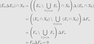
and so . Therefore

which shows that is indeed a measure.

Measurable Subspaces I

WordPress seems to have cleaned up its mess for now, so I’ll try to catch up.

When we’re considering the category of measurable spaces it’s a natural question to ask whether a subset of a measurable space is itself a measurable space in a natural way, and if this constitutes a subobject in the category. Unfortunately, unlike we saw with topological spaces, it’s not always possible to do this with measurable spaces. But let’s see what we can say.

Every subset comes with an inclusion function . If this is a measurable function, then it’s clearly a monomorphism; our question comes down to whether the inclusion is measurable in the first place. And so — as we did with topological spaces — we consider the preimage of a measurable subset . That is, what points satisfy ? Clearly, these are the points in the intersection . And so for to be measurable, we must have be measurable as a subset of .

An easy way for this to happen is for itself to be measurable as a subset of . That is, if , then for any measurable , we have . And so we can define to be the collection of all measurable subsets of that happen to fall within . That is, if and only if and . If is a measure space, with measure , then we can define a measure on by setting . This clearly satisfies the definition of a measure.

Conversely, if is a measure space and , we can make into a measure space ! A subset is in if and only if , and we define for such a subset .

As a variation, if we already have a measurable space we can restrict it to the measurable subspace . If we then define a measure on , we can extend this measure to a measure on by the same definition: , even though this is not the same one as in the previous paragraph.

Things break down

WordPress seems to have messed with again, and fouled it all up. Dozens of perfectly well-formed expressions are throwing errors, including $ latex \sigma$. Since writing lowercase sigmas is pretty much essential for the current topics, I’m just not going to write until they fix their mess.

And if anyone from WordPress reads this: one of the major I encouraged people to start math, physics, and computer science oriented weblogs on WordPress’ platform is exactly its support for LaTeX. It really annoys me to no end that you keep screwing with it and breaking it in pretty severe ways.

Measurable Spaces, Measure Spaces, and Measurable Functions

We’ve spent a fair amount of time discussing rings and -rings of sets, and measures as functions on such collections. Now we start considering how these sorts of constructions relate to each other.

A “measurable space” is some set and a choice of a -ring of subsets of . We call the members of the “measurable sets” of the measurable space. This is not to insinuate that is the collection of sets measurable by some outer measure , nor even that we can define a nontrivial measure on in the first place. Normally we just call the measurable space by the same name as the underlying set and omit explicit mention of .

Since it would be sort of silly to have points that can’t be discussed, we add the assumption that every point of is in some measurable set. Commonly, it’s the case that itself is measurable — — but we won’t actually require that be a -algebra.

A “measure space” is a measurable space along with a choice of a measure on the -ring . As before, we will usually call a measure space by the same name as the underlying set and omit explicit mention of the -ring and measure. Measure spaces inherit adjectives from their measures; a measure space is called finite, or -finite, or complete if its measure is finite, -finite, or complete, respectively.

Given a measure space , we will routinely use without comment the associated outer measure and inner measure on the hereditary -ring .

As an underlying set equipped with a particular collection of “special” subsets, a measurable space should remind us of a topological space, and like topological spaces they form a category. Remember that our original definition of a continuous function: given topological spaces and , a function is continuous if the preimage of any open set is open — for any we have .

We define a “measurable function” similarly: given measurable spaces and , a function is measurable if the preimage of any measurable set is measurable — for any we have . It’s straightforward to verify that the collection of measurable spaces and measurable functions forms a category. We will set this category in its full generality aside for the moment, as is the usual practice in measure theory, but we will refer to it if appropriate to illuminate a point.

Before I close, though, I’d like to put out a question that I don’t know the answer to, and which some friends haven’t really been able to answer when I mused about it in front of them. When we dealt with topology, we were able to recast the basic foundations in terms of nets. That is, a function is continuous if and only if it “preserves limits of convergent nets” — if it sends any convergent net in the domain to another convergent net in the range, and the action of the function commutes with passage to the limit. I like this because the idea of “preserving” some structure (albeit an infinite and often-messy one) feels more natural and algebraic that the idea of inspecting preimages of open sets. And so I put the question out to the audience: what is “preserved” by a measurable function, in the same way that continuous functions preserve limits of convergent nets?

Non-Lebesgue Measurable Sets

I need to make up for missing a post earlier this week…

The most important observation about the fact that Lebesgue measurable sets might not be all of is sort of tautological: it means that there may be subsets of the real line which are not Lebesgue measurable. That is, sets for which it is impossible to give a sense of “how much space they take up”, in a way compatible with the length of an interval.

And we can show that such sets do, in fact, exist. At least, we can build them if we have use of the axiom of choice. This might seem like a reason not to use the axiom of choice, but remember that Zorn’s lemma — which is equivalent to the axiom of choice — was essential when we needed to show that every vector space has a basis, or Tychonoff’s theorem, or that exact sequences of vector spaces split. So it’s sort of a mixed bag. In practice, most working mathematicians seem to be willing to accept the existence of non-Lebesgue measurable sets in order to gain the above benefits.

So, first a lemma: if is irrational, then the set of all numbers of the form with and any integers is dense in the real line. That is, every open interval contains at least one point of . The same is true for the set where we restrict to be even, and for the set where we restrict to be odd. Note (and, incidentally, ) is actually a subgroup of the additive group of real numbers.

For every integer there is some unique integer so that ; we will write . If is an open interval, there is some positive integer with . Picking out the first numbers , there must be some pair and with (or else they wouldn’t all fit in the interval ). But then some multiple of must land within , as we asserted. For , we can do the same using the interval , and for we can use the fact that .

Now, I say that there exists at least one set which is not Lebesgue measurable. To show this, we consider the quotient group . That is, we use an equivalence relation if . This divides up the real numbers into a disjoint union of equivalence classes under this relation, and the axiom of choice allows us to build a set by picking exactly one point from each equivalence class. This is the set we will show is not Lebesgue measurable.

Suppose is a Borel set contained in . The difference set contains no point of , since if this happened we’d have two points in picked from the same -equivalence class. But we just saw that any open interval contains a point of , and so our result from last time shows that must have outer measure zero — if it had positive outer measure then would contain an open interval. And so if is Lebesgue measurable then its Lebesgue measure must be zero.

Now if and are distinct elements of , then and must be disjoint. As we let range over the countable number of values in , the sets then form a countable disjoint cover of . But each of the is just a translation of , and so each one must have the same measure. And then since Lebesgue measure is countably additive, we must have

But this is clearly nonsense.

We can do even better, actually, in our efforts to find bizarre sets. There exists a subset so that for every Lebesgue measurable set we have both

That is, no matter what Lebesgue measurable set we pick, its intersection with is so weird that no set of positive Lebesgue measure can fit inside it, and yet itself is the smallest Lebesgue measurable sets that can contain it.

To find this set, write from our lemma and take to the set we just constructed. Define — the set of sums of points in and points in . If is a Borel set contained in , then can’t contain any point of (using a similar argument to that from earlier). And so we must have .

On the other hand, we just saw that , and thus

And so as well. If is any Lebesgue measurable set, the monotonicity of gives us . And then an earlier result tells us that

Lebesgue Measurable Sets

The attentive reader will note that in our study of Lebesgue measure we’ve defined it on some complete -algebra . In general, there’s no reason to believe that such a -algebra would be all of , and so there’s some interesting structure worth investigating. Our intuition is amazingly bad at conceiving of just how bizarre and perverse a “general” subset of the real line can be, and so the facts we learn about Lebesgue measurable sets seem sort of opaque when we first see them, but they will turn out to be useful.

First, let’s recall where they come from. There’s an outer measure associated with Lebesgue measure , and then there is the collection of sets measurable by . These are the sets so that for any subset we have

If is a Lebesgue measurable set of positive, finite measure, and if is a real number, then there exists some open interval so that

That is, Lebesgue measurable sets do a pretty good job of covering sections of the real line. If we think of as a measure of efficiency, we can always find some interval so that covers at least that portion of it.

Let is the class of open sets. We already know that

So we can find some open containing and satisfying . This will be the disjoint union of a sequence of open intervals , and so it follows that

We must have for at least one of these summands, and this gives us the we were looking for.

If is again a Lebesgue measurable set with positive measure, then there exists an open interval containing and entirely contained in the set of “differences” in . That is, the set defined by

If contains an open interval itself, then this is trivially true. We can just take the desired interval to be , which clearly falls into the difference set . But general Lebesgue measurable sets don’t contain open intervals. And yet this is not just a collection of scattered points, because then it would have measure zero. We have points clustered closely enough to fill up area, but not enough to actually fill out any open intervals. This is, in fact, supremely weird if you really think about it.

But even if doesn’t fill up an interval, it comes close! The above result tells us that we can find a so that

Now pick some . Take the set , slide it over by adding to every point in the set, and call the result . The set is now contained in an open interval — — whose length is less than . If and were disjoint, then they’d have to have the same measure, and their union would have measure greater than and wouldn’t fit into this interval. So and must overlap a bit.

But this tells us that there’s a point that’s equal to the point . Thus is a point in . And so contains the whole interval , as we wanted.

Lebesgue Measure and Affine Transformations

This didn’t make it up yesterday, due to some preoccupation on my part. Playing catch-up…

The thing that makes Lebesgue measure really special is the way that every part of the real line “looks like” every other part, and the same is true as we scale the line up or down. Once we specify the measure of one interval then the measure of every other interval — and every Lebesgue measurable set — is completely determined. But first, let’s show that this nice behavior actually holds.

Let be an affine transformation of the real line, defined by for some real and any real . This is invertible, and the inverse function is affine as well: . Given a subset , we write for the image of under the transformation — . I say that the outer and inner Lebesgue measures are both nicely behaved under the transformation .

We’ll start by assuming that . In the other case, is the composition of the mapping and an affine transformation with a positive multiplier, so we’ll have to come back and show that this reflection preserves our measures.

Let be the collection of all sets of the form with . It should be clear that this is a -ring, and we will show that . Indeed, if is a semiclosed interval , then , where is the semiclosed interval . And so , and the whole -ring generated by must be contained in : . We can apply the exact same reasoning to to conclude that , and thus . This shows that .

For every Borel set , we define and . These are both measures on . If is a semiclosed interval, we calculate

so the two measures agree on . But our extension theorem tells us that a measure on is uniquely determined by its values on . And thus our assertion holds for Lebesgue measure on Borel sets.

Now if we apply these considerations to , we can show that

Replacing by and by , we also reach our conclusion for inner Lebesgue measure. But we still need to verify that preserves Lebesgue measurability in the first place. If is Lebesgue measurable, and is any set, then

and thus is also Lebesgue measurable.

Now let’s go back and consider what happens with the reflection . This sends the semiclosed interval to the interval . But this is a Borel set: , and the singletons are Borel sets. Thus we see that the reflection sends Borel sets to Borel sets. It should also be clear that it preserves Lebesgue measure, for . If is a subset of a Borel set of measure zero, then the reflection of is again such a subset, and so we see that reflection preserves the Lebesgue measurable sets as well as their inner and outer measures.

Borel Sets and Lebesgue Measure

Let’s consider some of the easy properties of the Borel sets and Lebesgue measure we introduced yesterday.

First off, every countable set of real numbers is a Borel set of measure zero. In particular, every single point is a Borel set. Indeed, can be written as the countable intersection

so it’s a Borel set. Further, monotonicity tells us that

and so the singleton has measure zero. But is countably additive, so given any countable collection the measure is the sum of the measures of the individual points, each of which is zero.

Next, as I said when I introduced semiclosed intervals, we could have started with open intervals, but the details would have been messier. Now we can see that the -ring generated by the collection of semiclosed intervals is the same as that generated by the collection of all open sets.

We can see, in particular, that each open interval is a Borel set. Indeed, the point is a Borel set, as is the semiclosed interval , and we have the relation . Every other open set in is a countable union of open intervals, and so they’re all Borel sets as well. Conversely, we could write

and find the singleton in the -ring generated by . Then we can write and find every semiclosed interval in this -ring as well. And thus

We can also tie our current measure back to the concept of outer Lebesgue measure we introduced before. Back then, we defined the “volume” of a collection of open intervals to be the sum of the “volumes” of the intervals themselves. We defined the outer measure of a set to be the infimum of the volumes of finite open covers. And, indeed, this is exactly the outer measure corresponding to Lebesgue measure .

Remember that the outer measure is defined for a set by

Since , we have the inequality

On the other hand, if is any positive number, then by the definition of we can find a sequence of semiclosed intervals so that

and

We can thus widen each of these semiclosed intervals just a bit to find

and

Since was arbitrary, we find that . And, thus, that

In effect, we’ve replaced the messily-defined “volume” of an open cover by the more precise Lebesgue measure , but the result is the same. The “outer Lebesgue measure” from our investigations of multiple integrals is the same as the outer measure induced by our new Lebesgue measure.