Local Rings

Sorry for the break last Friday.

As long as we’re in the neighborhood — so to speak — we may as well define the concept of a “local ring”. This is a commutative ring which contains a unique maximal ideal. Equivalently, it’s one in which the sum of any two noninvertible elements is again noninvertible.

Why are these conditions equivalent? Well, if we have noninvertible elements and with invertible, then these elements generate principal ideals and . If we add these two ideals, we must get the whole ring, for the sum contains , and so must contain , and thus the whole ring. Thus and cannot both be contained within the same maximal ideal, and thus we would have to have two distinct maximal ideals.

Conversely, if the sum of any two noninvertible elements is itself noninvertible, then the noninvertible elements form an ideal. And this ideal must be maximal, for if we throw in any other (invertible) element, it would suddenly contain the entire ring.

Why do we care? Well, it turns out that for any manifold and point the algebra of germs of functions at is a local ring. And in fact this is pretty much the reason for the name “local” ring: it is a ring of functions that’s completely localized to a single point.

To see that this is true, let’s consider which germs are invertible. I say that a germ represented by a function is invertible if and only if . Indeed, if , then is certainly not invertible. On the other hand, if , then continuity tells us that there is some neighborhood of where . Restricting to this neighborhood if necessary, we have a representative of the germ which never takes the value zero. And thus we can define a function for , which represents the multiplicative inverse to the germ of .

With this characterization of the invertible germs in hand, it should be clear that any two noninvertible germs represented by and must have . Thus , and the germ of is again noninvertible. Since the sum of any two noninvertible germs is itself noninvertible, the algebra of germs is local, and its unique maximal ideal consists of those functions which vanish at .

Incidentally, we once characterized maximal ideals as those for which the quotient is a field. So which field is it in this case? It’s not hard to see that — any germ is sent to its value at , which is just a real number.

Specifying Morphisms Between Boolean Rings

It will be useful to have other ways of showing that a given function between boolean rings is a morphism. The definition, of course, is that and , since and here denote our addition and multiplication, respectively.

It’s also sufficient to show that and . Indeed, we can build both and from and :

So if and are preserved, then so are and .

A little more subtle is the fact that for surjections we can preserve order in both directions. That is, if is equivalent to for a surjection from one underlying set onto the other, then is a homomorphism of Boolean rings. We first show that preserves by using its characterization as a least upper bound: , , and if and then .

So, since preserves order, we know that , and that . We can conclude from this that , and we are left to short that . But f(E)\cup f(F)=f(G)$ for some , since is surjective. Since , we must have , and similarly . But then , and so , as we wanted to show.

We thus know that preserves the operation , and we can similarly show that preserves , using the dual universal property. In order to build and from and , we need complements. But complements satisfy a universal property of their own: , and if then .

First, I want to show that by showing it is below all elements of . Indeed, by the surjectivity of , every element of is the image of some element . Thus we want to show that . But this is true because for all , and so

Now given a set and its complement , we know that . Since preserves , we must have . Let’s say is another set so that . By the surjectivity of , we have for some . Thus , and thus . This tells us that , and thus . And so .

Therefore, since preserves , , and complements, it preserves and , and thus is a morphism of Boolean rings.

Completeness of Boolean Rings

We have a notion of “completeness” for boolean rings, which is related to the one for uniform spaces (and metric spaces), but which isn’t quite the same thing. We say that a Boolean ring is complete if every set of elements of has a union.

A complete Boolean ring is clearly a Boolean -algebra. It’s an algebra, because we can get a top element by taking the union of all the elements of together, and it’s a -ring because countable unions are included under all unions. The converse is a little hairier.

First off, every totally finite measure algebra is complete. That is, if — and thus for all , then every collection of elements of will have a union.

We let be the collection of all finite unions of elements in , all of which exist since is a Boolean ring. We let be the (finite) supremum of the measures of all elements in . Since this is a finite supremum, there must be some increasing sequence so that increases to . I say that the union of the sequence — which exists because is a -ring — is the union of all of .

Indeed, we must have by the continuity of the measure . Take any set and consider the difference , which is the amount by which extends past . Our assertion is that this is always . Define the sets , which is a disjoint union since is disjoint from . Each of the is in , and the limit of the sequence is . This set has measure

but since each of the is bounded above by then so is their limit. Thus , and thus , since we consider all negligible sets to be the same.

The same is true for totally -finite measure algebras. Indeed, we can break such a measure algebra up into a countable collection of finite measure algebras by breaking into a countable number of elements so that . We define the finite measure algebra to consist of the intersections of elements of with . Then given any collection we consider its image under such intersections to get . What we said above shows that each of these collections has an intersection , and their union in is the union of the original collection .

Functions on Boolean Rings and Measure Rings

We’re not just interested in Boolean rings as algebraic structures, but we’re also interested in real-valued functions on them. Given a function on a Boolean ring , we say that is additive, or a measure, -finite (on -rings), and so on analogously to the same concepts for set functions. We also say that a measure on a Boolean ring is “positive” if it is zero only for the zero element of the Boolean ring.

Now, if is the Boolean -ring that comes from a measurable space , then usually a measure on is not positive under this definition, since there exist sets of measure zero. However, remember that in measure theory we usually talk about things that happen almost everywhere. That is, we consider two sets — two elements of — to be “the same” if their difference is negligible — if the value of takes the value zero on this difference. If we let be the collection of -negligible sets, it turns out that is an ideal in the Boolean -ring . Indeed, if and are negligible, then so is , so is an Abelian subgroup. Further, if and , then , so is an ideal.

So we can form the quotient ring , which consists of the equivalence classes of elements which differ by an element of measure zero. This is equivalent to our old rhetorical trick of only considering properties up to “almost everywhere”. Using this new definition of “equals zero”, any measure on a Boolean -ring gives rise to a positive measure on the quotient -ring . In particular, given a measure space , we write for the Boolean -ring it gives rise to.

We say that a “measure ring” is a Boolean -ring together with a positive measure on . For instance, if is a measure space, then is a measure ring.. If is a Boolean -algebra we say that is a measure algebra. We say that measure rings and algebras are (totally) finite or -finite the same as for measure spaces. Measure rings, of course, form a category; a morphism from one measure algebra to another is a morphism of boolean -algebras so that for all .

I say that the mapping which sends a measure space to its associated measure algebra is a contravariant functor. Indeed, let be a morphism of measure spaces. That is, is a measurable function from to , so contains the pulled-back -algebra . This pull-back defines a map . Further, since is a morphism of measure spaces it must push forward to . That is, , or in other words . And so if then , thus the ideal is sent to the ideal , and so descends to a homomorphism between the quotient rings: . As we just said, , and thus we have a morphism of measure algebras . It’s straightforward to confirm that this assignment preserves identities and compositions.

Boolean Rings

A “Boolean ring” is a commutative ring with the additional property that each and every element is idempotent. That is, for any we have . An immediate consequence of this axiom is that , since we can calculate

The typical example we care about in the measure-theoretic context is a ring of subsets of some set , with the operation for addition and for multiplication. You should check that these operations satisfy the axioms of a Boolean ring. Since this is our main motivation, we will just consistently use and to denote addition and multiplication in Boolean rings, whether they arise from a measure theoretic context or not. From here it looks a lot like set theory, but keep in mind that the objects we’re looking at may have nothing to do with sets.

We can use these operations to define the other common set-theoretic operations. Indeed

and

and we can then define orders in the usual manner: .

As usual, the union of two elements is the “smallest” (with respect to this order) element above both of them, and the intersection of two elements is the “largest” element below both of them. The same goes for any finite number of elements, but if we try to move to an infinite number of elements there is no guarantee that there is any element above or below all of them, much less that such an element is unique. A “Boolean -ring” is a Boolean ring so that every countably infinite set of elements has a union. In this case, it is immediately true that any countably infinite set of elements has an intersection as well. The typical example, of course, is a -ring of subsets of a set .

A “Boolean algebra” is a Boolean ring for which there is some element so that for all elements . A “Boolean -algebra” is both a Boolean -ring and a Boolean algebra.

In the obvious way we have a full subcategory of the category of rings. It contains full subcategories of Boolean -rings, Boolean algebras, and Boolean -algebras.

Graded Objects

We’re about to talk about certain kinds of algebras that have the added structure of a “grading”. It’s not horribly important at the moment , but we might as well talk about it now so we don’t forget later.

Given a monoid , a -graded algebra is one that, as a vector space, we can write as a direct sum

so that the product of elements contained in two grades lands in the grade given by their product in the monoid. That is, we can write the algebra multiplication by

for each pair of grades and . As usual, we handle elements that are the sum of two elements with different grades by linearity.

By far the most common grading is by the natural numbers under addition, in which case we often just say “graded”. For example, the algebra of polynomials is graded, where the grading is given by the total degree. That is, if is the algebra of polynomials in variables, then the grade consists of sums of products of of the variables at a time. This is a grading because the product of two such homogeneous polynomials is itself homogeneous, and the total degree of each term in the product is the sum of the degrees of the factors. For instance, the product of in grade and 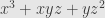in grade is

in grade .

Other common gradings include -grading and -grading. The latter algebras are often called “superalgebras”, related to their use in studying supersymmetry in physics. “Superalgebra” sounds a lot more big and impressive than “-graded algebra”, and physicists like that sort of thing.

In the context of graded algebras we also have graded modules. A -graded module over the -graded algebra can also be written down as a direct sum

But now it’s the action of on that involves the grading:

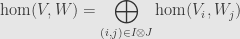
We can even talk about grading in the absence of a multiplicative structure, like a graded vector space. Now we don’t even really need the grades to form a monoid. Indeed, for any index set we might have the graded vector space

This doesn’t seem to be very useful, but it can serve to recognize natural direct summands in a vector space and keep track of them. For instance, we may want to consider a linear map between graded vector spaces and that only acts on one grade of and with an image contained in only one grade of :

We’ll say that such a map is graded . Any linear map from to can be decomposed uniquely into such graded components

giving a grading on the space of linear maps.

The Category of Representations

Now let’s narrow back in to representations of algebras, and the special case of representations of groups, but with an eye to the categorical interpretation. So, representations are functors. And this immediately leads us to the category of such functors. The objects, recall, are functors, while the morphisms are natural transformations. Now let’s consider what, exactly, a natural transformation consists of in this case.

Let’s say we have representations and 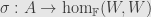. That is, we have functors and with , — where is the single object of , when it’s considered as a category — and the given actions on morphisms. We want to consider a natural transformation .

Such a natural transformation consists of a list of morphisms indexed by the objects of the category . But has only one object: . Thus we only have one morphism, , which we will just call .

Now we must impose the naturality condition. For each arrow in we ask that the diagram

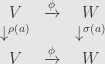
commute. That is, we want for every algebra element . We call such a transformation an “intertwiner” of the representations. These intertwiners are the morphisms in the category of of representations of . If we want to be more particular about the base field, we might also write .

Here’s another way of putting it. Think of as a “translation” from to . If is an isomorphism of vector spaces, for instance, it could be a change of basis. We want to take a transformation from the algebra and apply it, and we also want to translate. We could first apply the transformation in , using the representation , and then translate to . Or we could first translate from to and then apply the transformation, now using the representation . Our condition is that either order gives the same result, no matter which element of we’re considering.

Algebra Representations

We’ve defined a representation of the group as a homomorphism 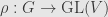for some vector space . But where did we really use the fact that is a group?

This leads us to the more general idea of representing a monoid . Of course, now we don’t need the image of a monoid element to be invertible, so we may as well just consider a homomorphism of monoids 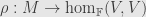, where we consider this endomorphism algebra as a monoid under composition.

And, of course, once we’ve got monoids and -linearity floating around, we’re inexorably drawn — Serge would way we have an irresistable compulsion — to consider monoid objects in the category of -modules. That is: –algebras.

And, indeed, things work nicely for -algebras. We say a representation of an -algebra is a homomorphism for some vector space over . How else can we view such a homomorphism?

Well, it turns an algebra element into an endomorphism. And the most important thing about an endomorphism is that it does something to vectors. So given an algebra element , and a vector , we get a new vector . And this operation is -linear in both of its variables. So we have a linear map , built from the representation and the evaluation map . But this is just a left –module!

In fact, the evaluation above is the counit of the adjunction between and the internal functor . This adjunction is a natural isomorphism of sets: . That is, left -modules are in natural bijection with representations of . In practice, we just consider the two structures to be the same, and we talk interchangeably about modules and representations.

As it would happen, the notion of an algebra representation properly extends that of a group representation. Given any group we can build the group algebra . As a vector space, this has a basis vector for each group element . We then define a multiplication on pairs of basis elements by , and extend by bilinearity.

Now it turns out that representations of the group and representations of the group algebra are in bijection. Indeed, the basis vectors are invertible in the algebra . Thus, given a homomorphism , the linear maps must be invertible. And so we have a group representation . Conversely, if is a representation of the group , then we can define and extend by linearity to get an algebra representation .

So we have representations of algebras. Within that we have the special cases of representations of groups. These allow us to cast abstract algebraic structures into concrete forms, acting as transformations of vector spaces.

The Exponential Series

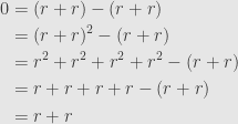
What is it that makes the exponential what it is? We defined it as the inverse of the logarithm, and this is defined by integrating . But the important thing we immediately showed is that it satisfies the exponential property.

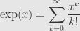
But now we know the Taylor series of the exponential function at :

In fact, we can work out the series around any other point the same way. Since all the derivatives are the exponential function back again, we find

Or we could also write this by expanding around and writing the relation as a series in the displacement :

Then we can expand out the part as a series itself:

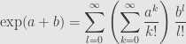
But then (with our usual handwaving about rearranging series) we can pull out the inner series since it doesn’t depend on the outer summation variable at all:

And these series are just the series defining and , respectively. That is, we have shown the exponential property directly from the series expansion.

That is, whatever function the power series defines, it satisfies the exponential property. In a sense, the fact that the inverse of this function turns out to be the logarithm is a big coincidence. But it’s a coincidence we’ll tease out tomorrow.

For now I’ll note that this important exponential property follows directly from the series. And we can write down the series anywhere we can add, subtract, multiply, divide (at least by integers), and talk about convergence. That is, the exponential series makes sense in any topological ring of characteristic zero. For example, we can define the exponential of complex numbers by the series

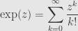
Finally, this series will have the exponential property as above, so long as the ring is commutative (like it is for the complex numbers). In more general rings there’s a generalized version of the exponential property, but I’ll leave that until we eventually need to use it.

The Taylor Series of the Exponential Function

Sorry for the lack of a post yesterday, but I was really tired after this weekend.

So what functions might we try finding a power series expansion for? Polynomials would be boring, because they already are power series that cut off after a finite number of terms. What other interesting functions do we have?

Well, one that’s particularly nice is the exponential function . We know that this function is its own derivative, and so it has infinitely many derivatives. In particular, , , , …, , and so on.

So we can construct the Taylor series at . The coefficient formula tells us

which gives us the series

We use the ratio test to calculate the radius of convergence. We calculate

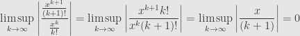
Thus the series converges absolutely no matter what value we pick for . The radius of convergence is thus infinite, and the series converges everywhere.

But does this series converge back to the exponential function? Taylor’s Theorem tells us that

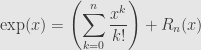
where there is some between and so that .

Now the derivative of is again, and takes only positive values. And so we know that is everywhere increasing. What does this mean? Well, if then , and so . On the other hand if then , and so . Either way, we have some uniform bound on no matter what the are.

So now we know . And it’s not too hard to see (though I can’t seem to find it in my archives) that grows much faster than for any fixed . Basically, the idea is that each time you’re multiplying by , which eventually gets less than and stays less than one. The upshot is that the remainder term must converge to for any fixed , and so the series indeed converges to the function .