The Unapologetic Mathematician

Mathematics for the interested outsider

Natural Transformations and Functor Categories

So we know about categories and functors describing transformations between categories. Now we come to transformations between functors — natural transformations.

This is really what category theory was originally invented for, and the terminology predates the theory. Certain homomorphisms were called “natural”, but there really wasn’t a good notion of what “natural” meant. In the process of trying to flesh that out it became clear that we were really talking about transformations between the values of two different constructions from the same source, and those constructions became functors. Then in order to rigorously define what a functor was, categories were introduced.
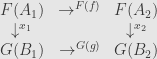
Given two functors F:\mathcal{C}\rightarrow\mathcal{D} and G:\mathcal{C}\rightarrow\mathcal{D}, a natural transformation \eta:F\rightarrow G is a collection of arrows \eta_C:F(C)\rightarrow G(C) in \mathcal{D} indexed by the objects of \mathcal{C}. The condition of naturality is that the following square commutes for every arrow f:A\rightarrow B in \mathcal{C}:

\begin{matrix}F(A)&\rightarrow^{\eta_A}&G(A)\\\downarrow^{F(f)}&&\downarrow^{G(f)}\\F(B)&\rightarrow^{\eta_B}&G(B)\end{matrix}

The vertical arrows from from applying the two functors to the arrow f, and the horizontal arrows are the components of the natural transformation.

If we have three functors F, G, and H from \mathcal{C} to \mathcal{D} and natural transformations \eta:F\rightarrow G and \xi:G\rightarrow H we get a natural transformation \xi\circ\eta:F\rightarrow H with components (\xi\circ\eta)_C=\xi_C\circ\eta_C. Indeed, we can just stack the naturality squares beside each other:

\begin{matrix}F(A)&\rightarrow^{\eta_A}&G(A)&\rightarrow^{\xi_A}&H(A)\\\downarrow^{F(f)}&&\downarrow^{G(f)}&&\downarrow^{H(f)}\\F(B)&\rightarrow^{\eta_B}&G(B)&\rightarrow^{\xi_B}&H(B)\end{matrix}

and the outer square commutes because both the inner ones do.

Every functor comes with the identity natural transformation 1_F, whose components are all identity morphisms. Clearly it acts as the identity for the above composition of natural transformations.

A natural transformation is invertible for the above composition if and only if each component is invertible as an arrow in \mathcal{D}. In this case we call it a “natural isomorphism”. We say two functors are “naturally isomorphic” if there is a natural isomorphism between them.

All of this certainly looks like we’re talking about a category, but again the set theoretic constraints often work against us. There are, however, times where we really do have a category. If one of \mathcal{C} or \mathcal{D} (or both) are small, then all the set theory works out and we get an honest category of functors from \mathcal{C} to \mathcal{D}. We will usually denote this category as \mathcal{D}^\mathcal{C}. Its objects are functors from \mathcal{C} to \mathcal{D}, and its morphisms are natural transformations between such functors.

And now we can explain the notation \mathcal{C}^\mathbf{2} for the category of arrows. This is the category of functors from \mathbf{2} to \mathcal{C}! What is a functor from \mathbf{2} to \mathcal{C}? Remember that \mathbf{2} is the category with two objects A and B and one non-trivial arrow f:A\rightarrow B. Thus a functor F:\mathbf{2}\rightarrow\mathcal{C} is defined by an arrow F(f):F(A)\rightarrow F(B), and there’s exactly one functor for every arrow in \mathcal{C}.

Now let’s say we have two such functors F(f):F(A)\rightarrow F(B) and G(f):G(A)\rightarrow G(B). A natural transformation \eta:F\rightarrow G consists of morphisms \eta_A:F(A)\rightarrow G(A) and \eta_B:F(B)\rightarrow G(B) so that the naturality square commutes. But this is the same thing we used to define morphisms in the arrow category, just with some different notation!

Natural transformations and functor categories show up absolutely everywhere once you know to look for them. We’ll be seeing a lot more examples as we go on.

May 26, 2007 Posted by | Category theory | 7 Comments

Comma Categories

Another useful example of a category is a comma category. The term comes from the original notation which has since fallen out of favor because, as Saunders MacLane put it, “the comma is already overworked”.

We start with three categories \mathcal{A}, \mathcal{B}, and \mathcal{C}, and two functors F:\mathcal{A}\rightarrow\mathcal{C} and G:\mathcal{B}\rightarrow\mathcal{C}. The objects of the comma category (F\downarrow G) are triples (A,x,B) where A is an object of \mathcal{A}, B is an object of \mathcal{B}, and x is an arrow F(A)\rightarrow G(B) in \mathcal{C}. The morphisms are pairs (f,g) — with f an arrow in \mathcal{A} and g an arrow in \mathcal{B} — making the following square commute:

\begin{matrix}F(A_1)&\rightarrow^{F(f)}&F(A_2)\\\downarrow^{x_1}&&\downarrow^{x_2}\\G(B_1)&\rightarrow^{G(g)}&G(B_2)\end{matrix}

So what? Well, let’s try picking F to be the functor A:\mathbf{1}\rightarrow\mathcal{A} sending the single object of \mathbf{1} to the object A\in\mathcal{A}. Then let \mathcal{G} be the identity functor on \mathcal{A}. Now an object of (A\downarrow1_\mathcal{A}) is an arrow f:A\rightarrow B, where B can be any other object in \mathcal{A}. A morphism is then a triangle:

\begin{matrix}A&&\\\downarrow^{f}&\searrow^{f'}&\\B&\rightarrow^{g}&B'\end{matrix}

Work out for yourself the category (1_\mathcal{A}\downarrow A).

Here’s another example: the category (1_\mathcal{A}\downarrow 1_\mathcal{A}). Verify that this is exactly the arrow category \mathcal{A}^\mathbf{2}.

And another: check that given objects A and B in \mathcal{A}, the category (A\downarrow B) is the discrete category (set) \hom_\mathcal{A}(A,B).

Neat!

May 26, 2007 Posted by | Category theory | 11 Comments