Today I want to run through a bunch of examples of the constructions we’ve been considering for modules. I’ll restrict to the case of a ring  with unit.
One easy example of an -module that I’ve mentioned before is the ring itself. We drop down to the underlying abelian group and then act on it using the ring multiplication. There are both left and right actions here:  and
and  where
where  and
and  are ring elements, considered as an element of the module. We’ll start off by taking this module and sticking it into some of the constructions.
When we consider  for some left -module
  the left module structures on and will get eaten and the right module structure on will get flipped over, leaving us a left -module. We can pick an element
  by specifying
  . Then
  , telling us where everything else goes. If we write
  for the homomorphism with
  , then the left action of on homomorphisms says
=f_m(r\cdot1)=r\cdot f_m(1)=r\cdot m](https://s0.wp.com/latex.php?latex=%5Cleft%5Br%5Ccdot+f_m%5Cright%5D%281%29%3Df_m%28r%5Ccdot1%29%3Dr%5Ccdot+f_m%281%29%3Dr%5Ccdot+m&bg=e6e6e6&fg=333333&s=0&c=20201002)
Thus  . This means that
  as left -modules.
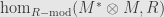
On the other hand, if we consider  we get a right -module. This consists of all -linear functions from to the ring itself. We call this the “dual” module to , and write
  . Elements of the dual module are often called “linear functionals” on .
Tensor products are even easier. When we consider  for a left -module we can use the construction of tensor products to write an element as a finite sum:
  . But then we can use the middle-linear property to write
  , and then the linearity to collect all the terms together, giving
  . The tensor product eats the module structure on and the right module structure on , leaving a left -module structure. We calculate

so  as left -modules.
Now let’s take two left -modules and  and make
  . This is an abelian group — a
  -module — as is . Let’s write as
  as above and then tensor over with . Then we can compose homomorphisms

This is the “evaluation” homomorphism that takes an element  and a homomorphism
  and gives back
  .
.
As a special case, we can take itself in place of . We get an evaluation homomorphism  . This “canonical pairing” we often write as
  for a linear functional
  and module element
  .
.
What if we composed with an element of  instead of
  ? We use the evaluation homomorphism to get

So given a homomorphism  we get a homomorphism
Of course, all this goes through suitably changed by swapping “right” for “left”. For example, given a right -module we have a dual left -module  .
.
What do we get if we start with a left module , dualize it, then dualize again to get another left module  ? Following the definitions we see
  . I claim that there is a natural morphism of left -modules
  . That is, a special element of

but we know that this is isomorphic to

which we write as
so we’re really looking for a special homomorphism from  to . And we’ve got one: the canonical pairing! So we take the canonical pairing as a homomorphism from and pass it through this natural isomorphism to get a homomorphism
  . In case this looks completely insane, here it is in terms of elements:
  takes a linear functional and gives back an element of the ring by the rule
 =\mu(m)](https://s0.wp.com/latex.php?latex=%5Cleft%5Bd%28m%29%5Cright%5D%28%5Cmu%29%3D%5Cmu%28m%29&bg=e6e6e6&fg=333333&s=0&c=20201002) .
.
May 4, 2007
Posted by John Armstrong |
Ring theory |
1 Comment
One interesting question for any partial order is that of lower or upper bounds. Given a partial order  and a subset
  we say that
  is a lower bound of
  if
if  for every element
  . Similarly, an upper bound is one so that
  for every
  .
.
A given subset may have many different lower bounds. For example, if is a lower bound for and  , then the transitive property of
  shows that
  is also a lower bound. If we’re lucky, we can find a greatest lower bound. This is a lower bound
  so that for any other lower bound we have
  . Then the set of all lower bounds is just the set of all elements below .
As an explicit example, let’s consider the partial order we get from the divisibility relation on integers. In this case, a greatest lower bound is better known as a greatest common divisor, and for any pair of natural numbers we can find a greatest common divisor. The method we use actually goes all the way back to Euclid’s Elements, proposition VII.2. Because of this, it’s known as Euclid’s algorithm.
First we need remember how we divide numbers from back in arithmetic. Given two numbers  and we can find numbers
  and with
  and
and  . We start with and make up all the natural numbers of the form
  with
with  a natural number. Since the natural numbers are well-ordered, there is a least element
  in this set. Notice that here we use the regular order on
  , not divisibility. Anyhow, I claim that is less than , so it will be our . Indeed if it’s greater than we can subtract from it to get
  : a lower natural number, which contradicts the fact that is the lowest. Thus we have found with . Notice that
  if and only if
  .
.
Okay, now that we remember how to divide we’re ready for Euclid’s algorithm. We start with numbers and and divide into to find  . If
. If  then and is a common divisor. It’s clearly the greatest since any common divisor divides it.
If  then I say that any common divisor of and
  is also a common divisor of and . We see that if
  and
and  then
then  so
so  as well. Thus if we can find the greatest common divisor of and it will also be the greatest common divisor of and .
To do this, just keep going. Divide into to get  . If
. If  then we’re done, otherwise keep going again. At each step
  , so we must eventually hit zero and stop. If we didn’t, then we could collect all the
  together to have a set of natural numbers with no lowest element, contradicting the well-ordered property of . At the end we’ll have the greatest common divisor of and .
In fact, if we watch closely we can do even better. We stop when  with a remainder of zero, getting the greatest common divisor
  . Now we look at the next-to-last step
 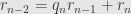 . We can rewrite this as
 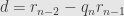 . Then the step before this —
  — can be written as
  . This gives us
  . We can keep doing this over and over, at each step writing as a linear combination of the two remainders that we started a given step with. Taking this all the way back to the beginning of the algorithm, we get
  for some integers and
  .
.
From here you should be able to see how to use Euclid’s algorithm to find the greatest common divisor of any finite set of natural numbers, and further how to write it as an integral linear combination of the elements of .
May 4, 2007
Posted by John Armstrong |
Ring theory |
3 Comments

