Roots of Polynomials II

This one might have to suffice for two days. The movers are almost done loading the truck here in New Orleans, and I’ll be taking today and tomorrow to drive to Maryland.

We can actually tease out more information from the factorization we constructed yesterday. Bur first we need a little definition.

Remember that when we set up the algebra of polynomials we noted that the coefficients have to be all zero after some finite number of them. Thus there must be a greatest nonzero coefficient . The index corresponding to this coefficient we call the “degree” of the polynomial. If all the coefficients are zero — giving the zero polynomial — then a common convention is to assign it degree . This actually isn’t completely arbitrary, but the details won’t concern us until later.

So, armed with this information, look at how we constructed the factorization . We replaced each term in with the term . Then we factored out from this term, giving . So the highest power of that shows up in this term (with a nonzero coefficient) is . And the highest power coming from all the terms of will be . The power shows up only once in the expression for , so there’s no way for two such terms to add together and make its coefficient turn out to be zero, and no higher power of ever shows up at all. Thus the degree of is one less than that of .

So what does this gain us? Well, each time we find a root we can factor out a term like , which reduces the degree by . So if has degree there can only be at most roots!

A nonzero constant polynomial has degree , but it also has no roots! Perfect.

A linear polynomial has degree , and it has exactly one root: .

Now let’s assume that our statement is true for all polynomials of degree : they have or fewer roots. Then given a polynomial of degree either has a root or it doesn’t. If it doesn’t, then we’re already done. If it does, then we can factor , where has degree . But then can have at most roots, and thus can have at most roots!

A nice little corollary of this is that if our base field is infinite (like it is for the most familiar examples) then only the zero polynomial can give us the zero function when we evaluate it at various field elements. That is, if for all , then . This must be true because has an infinite number of roots, and so no finite degree polynomial can possibly have that many roots. The only possibility left is the zero polynomial.

Just to be clear, though, let’s look at this one counterexample. Think about the field we used when we talked about Set. The polynomial is not the zero polynomial, but is the zero function. Indeed , , and , which is divisible by , and so is the same as in this field.

Roots of Polynomials I

When we consider a polynomial as a function, we’re particularly interested in those field elements so that . We call such an a “zero” or a “root” of the polynomial .

One easy way to get this to happen is for to have a factor of . Indeed, in that case if we write for some other polynomial then we evaluate to find

The interesting thing is that this is the only way for a root to occur, other than to have the zero polynomial. Let’s say we have the polynomial

and let’s also say we’ve got a root so that . But that means

This is not just a field element — it’s the zero polynomial! So we can subtract it from to find

Now for any we can use the identity

to factor out from each term above. This gives the factorization we were looking for.

Polynomials as Functions

When I set up the algebra of polynomials I was careful to specify that the element is not a “variable”, as in high school algebra. Why do I have to do that? What is the “variable” thing that we were all taught, then?

We’ve got the algebra of polynomials over the base field . Now I’m going to define a function called the “evaluation map”. We define by first writing out in terms of the standard basis

Remember here that the sum must terminate after a finite number of basis elements. Then we just stick the field element in for to get an expression written out in the field itself:

Now the superscripts on each must be read as exponents. This defines a particular element of the field. If we keep the polynomial fixed and let range over we get a function from to itself, which we can abuse notation to write as . This is the notion of polynomial-as-function we were taught in high school.

But it’s actually more interesting to see what happens as we fix and let vary over all polynomials. The map turns out to be a homomorphism of -algebras! Indeed, given polynomials

(the top coefficients here may be zero, and all higher coefficients definitely are) and a field element we find

I’ll let you write out the verification that it also preserves multiplication.

In practice this “evaluation homomorphism” provides a nice way of extracting information about polynomials. And considering polynomials as functions provides another valuable slice of information. But we must still keep in mind the difference between the abstract polynomial

and the field element

Polynomials

Okay, we’re going to need some other algebraic tools before we go any further into linear algebra. Specifically, we’ll need to know a few things about the algebra of polynomials. Specifically (and diverging from the polynomials discussed earlier) we’re talking about polynomials in one variable, and with coefficients in the field we’re building our vector spaces over already.

We’ll write this algebra as , where is now not a “variable”, like it was back in high school calculus. It’s a new element of the algebra. We start with the field which is trivially an algebra over itself. Then we just throw in this new thing called . Then, since we want to still be an algebra over , we have to be able to multiply elements. Defining a scalar multiple for each is a good start, but we also have to multiply by itself to get . There’s no reason this should be anything we’ve seen yet, so it’s new. Going along, we get , , and so on. Each of these is a new element, and we also get scalar multiples , and even linear combinations:

as long as there are only a finite number of nonzero terms in this sum. That is, the coefficients are all zero after some point. We customarily take — the unit of the algebra.

Note here that we’re not using the summation convention for polynomials, though we could in principle. Remember, an algebra is a vector space, and what we’ve said above establishes that the set constitutes a basis for this vector space!

The algebra structure can be specified by defining it on pairs of basis elements. Remember that the structure is just a bilinear multiplication, which is just a linear map from the tensor square to . And we know that the basis for a tensor product consists of pairs of basis elements. So we can specify this linear map on a basis and extend by linearity — bilinearity — whatever…

Anyhow, how should we define the multiplication? Simply: . Then the whole rest of the algebra structure is defined for us. Now this looks like adding exponents, but remember we can just as well think of these as indices on basis elements that just happen to add when we multiply corresponding basis elements. Thus we wouldn’t be out of place using the summation convention here, though we won’t for the moment.

Open Gap Thread

I’m preparing for my drive tomorrow. I’m heading down to New Orleans for the final move-out. As such, I think I’ll throw this one out to discuss the (non)existence of the math gender gap. Also, feel free to weigh in about Title IX applying to math and science departments. The latter I heard about through Jesse Johnson, so here’s a tam-tip to him.

Talk amongst yourselves.

The Inclusion-Exclusion Principle

In combinatorics we have a method of determining the cardinality of unions in terms of the sets in question and their intersection: the Inclusion–Exclusion Principle. Predictably enough, this formula is reflected in the subspaces of a vector space. We could argue directly in terms of bases, but it’s much more interesting to use the linear algebra we have at hand.

Let’s start with just two subspaces and of some larger vector space. We’ll never really need that space, so we don’t need to give it a name. The thing to remember is that and might have a nontrivial intersection — their sum may not be direct.

Now we consider the sum of the subspaces. Every vector in is the sum of a vector in and a vector in . This tells us that there’s a linear map defined by . Note carefully that this is linear as a function of the pair . It’s not bilinear — linear in each of and separately — which would mean bringing in the tensor product.

This function is always surjective, but it may fail to be injective. Specifically, if and have a nontrivial intersection then it gives us a nontrivial kernel. If then . But rather than talk about elements, let’s use the intersection to parametrize the kernel! We’ve got another linear map , defined by .

Now it’s clear that has a trivial kernel. On the other hand, its image is precisely the set of pairs that kills off. That means we’ve got an exact sequence:

Taking the Euler characteristic we find that

Some simple juggling turns this into

which is the inclusion-exclusion principle for two subspaces.

What about three subspaces , , and ? We start off again with

defined by . Then the kernel contains triples like , , and . We use the pairwise intersections to cover the kernel by the map

defined by . The image of is exactly the kernel of , but this time it has a nontrivial kernel itself! Now we need another map

defined by . Now is injective, and its image is exactly the kernel of . We stick these maps all together to have the long exact sequence

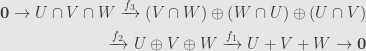
Taking the Euler characteristic and juggling again we find

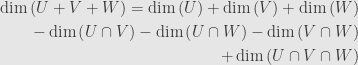
We include the dimensions of the individual subspaces, exclude the dimensions of the pairwise intersections, and include back in the dimension of the triple intersection.

For larger numbers of subspaces we can construct longer and longer exact sequences. The th term consists of the direct sum of the intersections of the subspaces, taken at a time. The th map consists of including each -fold intersection into each of the -fold intersections it lies in, with positive and negative signs judiciously sprinkled throughout to make the sequence exact.

The result is that the dimension of a sum of subspaces is the alternating sum of the dimensions of the -fold intersections. First add the dimension of each subspace, then subtract the dimension of each pairwise intersection, then add back in the dimension of each triple intersection, and so on.

From here it’s the work of a moment to derive the combinatorial inclusion-exclusion principle. Given a collection of sets, just construct the free vector space on each of them. These free vector spaces will have nontrivial intersections corresponding to the nonempty intersections of the sets, and we’ve got canonical basis elements floating around to work with. Then all these dimensions we’re talking about are cardinalities of various subsets of the sets we started with, and the combinatorial inclusion-exclusion principle follows. Of course, as I said before we could have proved it from the other side, but that would require a lot of messy hands-on work with bases and such.

The upshot is that the combinatorial inclusion-exclusion principle is equivalent to the statement that exact sequences of vector spaces have trivial Euler characteristic! This little formula that we teach in primary or secondary school turns out to be intimately connected with one of the fundamental tools of homological algebra and the abstract approach to linear algebra. Neat!

The Euler Characteristic of an Exact Sequence Vanishes

Naturally, one kind of linear map we’re really interested in is an isomorphism. Such a map has no kernel and no cokernel, and so its index is definitely zero. If it weren’t clear enough already, this shows that isomorphic vector spaces have the same dimension!

But remember that in abelian categories we’ve got diagrams to chase and exact sequences to play with. And these have something to say about the matters at hand.

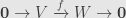
First, remember that a linear map whose kernel vanishes looks like this in terms of exact sequences:

And one whose cokernel vanishes looks like this:

So an isomorphism is just an exact sequence like this:

And then we have the equation

Yes, I’m writing the negative of the index here, but there’s a good reason for it.

Now what if we have a segment of an exact sequence:

Considering the map allows us to break up as (since short exact sequences split). On the other hand, considering the map allows us to break up as . Exactness tells us that , which gives us the isomorphism .

Now the rank-nullity theorem says that , and similarly for all other linear maps. So we get — which expresses as the direct sum of one subspace of and one of . And each of those vector spaces has another part to hand off to the vector space on its other side, and so on!

What does this mean? It says that if we look at every other term of an exact sequence and take their direct sum, the result is the same whether we look at the odd or the even terms. More explicitly, let’s say we have a long exact sequence

Then we can decompose each term as either or — one for the even terms and the other for the odd terms. Then direct-summing everything up we have an isomorphism

which tells us that

But since direct sums add dimensions this means

And now we can just combine these sums:

Which generalizes the formula we wrote above in the case of an isomorphism. This alternating sum we call the “Euler characteristic” of a sequence, and we’ll be seeing a lot more of that sort of thing in the future. But here the major result is that for exact sequences we always get the value zero.

In fact, this amounts to a far-reaching generalization of the rank-nullity theorem. And that theorem, of course, is essential to the proof. Yet again we see this pattern of “bootstrapping” our way from a special case to a larger theorem. Despite some mathematicians being enamored of reductio ad absurdum, this induction from special to general has to be one of the most useful tools we keep running across.

The Index of a Linear Map

Today I want to talk about the index of a linear map , which I’ll motivate in terms of a linear system for some linear map .

One important quantity is the dimension of the kernel of . In terms of the linear system, this is the dimension of the associated homogenous system . If there are any solutions of the system under consideration, they will form an affine space of this dimension.

But the system is inhomogenous in general, and as such it might not have any solutions. Since every short exact sequence of vector spaces splits we can write . Then the vector will have some component in the image of , and some component in the complementary subspace . Note that is not canonical here. I’m just asserting that some such subspace exists so we can make this decomposition.

Now the condition that the system have any solutions is that the component of in vanishes. But we can pick some basis for and think of each component of with respect to each of those basis elements vanishing. That is, we must apply a number of linear conditions equal to the dimension of in order to know that the system has any solutions at all. And once it does, it will have of them.

But what happens if we quotient out by ? We get the cokernel , which must then be isomorphic to ! So the number of conditions we need to apply to is the dimension of the cokernel.

Now I’ll define the index of the linear map to be the difference between the dimension of the kernel and the dimension of the cokernel. In the more general case, if one of these dimensions is infinite we may get an infinite index. But often we’ll restrict to the case of “finite index” operators, where the difference works out to be a well-defined finite number. Of course, when dealing with linear systems it’s guaranteed to be finite, but there are a number of results out there for the finite index case. In fact, this is pretty much what a “Fredholm operator” is, if we ever get to that.

Anyhow, we’ve got this definition:

Now let’s add and subtract the dimension of the image of :

Clearly the dimension of the image and the dimension of the cokernel add up to the dimension of the target space. But notice also that the rank-nullity theorem tells us that the dimension of the kernel and the dimension of the image add up to the dimension of the source space! That is, we have the equality

What happened here? We started with an analytic definition in terms of describing solutions to a system of equations, and we ended up with a geometric formula in terms of the dimensions of two vector spaces.

What’s more, the index doesn’t really depend much on the particulars of at all. Any two linear maps between the same pair of vector spaces will have the same index! And this gives us a simple tradeoff: for every dimension we add to the space of solutions, we have to add a linear condition to restrict the vectors for which there are any solutions at all.

Alternately, what happens when we add a new equation to a system? With a new equation the dimension of the target space goes up, and so the index goes down. One very common way for this to occur is for the dimension of the solution space to drop. This gives rise to our intuition that each new equation reduces the number of independent solutions by one, until we have exactly as many equations as variables.

The Sum of Subspaces

We know what the direct sum of two vector spaces is. That we define abstractly and without reference to the internal structure of each space. It’s sort of like the disjoint union of sets, and in fact the basis for a direct sum is the disjoint union of bases for the summands.

Let’s use universal properties to prove this! We consider the direct sum , and we have a basis for and a basis for . But remember that the whole point of a basis is that vector spaces are free modules.

That is, there is a forgetful functor from to , sending a vector space to its underlying set. This functor has a left adjoint which assigns to any set the vector space of formal linear combinations of elements of . This is the free vector space on the basis , and when we choose the basis for a vector space we are actually choosing an isomorphism .

Okay. So we’re really considering the direct sum , and we’re asserting that it is isomorphic to . But we just said that constructing a free vector space is a functor, and this functor has a right adjoint. And we know that any functor that has a right adjoint preserves colimits! The disjoint union of sets is a coproduct, and the direct sum of vector spaces is a biproduct, which means it’s also a coproduct. Thus we have our isomorphism. Neat!

But not all unions of sets are disjoint. Sometimes the sets share elements, and the easiest way for this to happen is for them to both be subsets of some larger set. Then the union of the two subsets has to take this overlap into account. And since subspaces of a larger vector space may intersect nontrivially, their sum as subspaces has to take this into account.

First, here’s a definition in terms of the vectors themselves: given two subspaces and of a larger vector space , the sum will be the subspace consisting of all vectors that can be written in the form for and . Notice that there’s no uniqueness requirement here, and that’s because if and overlap in anything other than the trivial subspace we can add a vector in that overlap to and subtract it from , getting a different decomposition. This is precisely the situation a direct sum avoids.

Alternatively, let’s consider the collection of all subspaces of . This is a partially-ordered set, where the order is given by containment of the underlying sets. It’s sort of like the power set of a set, except that only those subsets of which are subspaces get included.

Now it turns out that, like the power set, this poset is actually a lattice. The meet is the intersection of subspaces, but the join isn’t their union. Indeed, the union of subspaces usually isn’t a subspace at all! What do we use instead? The sum, of course! It’s easiest to verify this with the algebraic definition of a lattice.

The lattice does have a top element (the whole space ) and a bottom element (the trivial subspace ). It’s even modular! Indeed, let , , and be subspaces with . Then on the one hand we consider , which is the collection of all vectors , where , , and . On the other hand we consider , which is collection of all vectors , where , , and . I’ll leave it to you to show how these two conditions are equivalent.

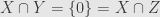
Unfortunately, the lattice isn’t distributive. I could work this out directly, but it’s easier to just notice that complements aren’t unique. Just consider three subspaces of : has all vectors of the form , has all of the form , and has all of the form . Then , and , but .

This is all well and good, but it’s starting to encroach on Todd’s turf, so I’ll back off a bit. The important bit here is that the sum behaves like a least-upper-bound.

In categorical terms, this means that it’s a product in the lattice of subspaces (considered as a category). Don’t get confused here! Direct sums are coproducts in the category , while sums are coproducts in the category (lattice) of subspaces of a given vector space. These are completely different categories, so don’t go confusing coproducts in one with those in the other.

In this case, all we mean by saying this is a categorical coproduct is that we have a description of the sum of two subspaces which doesn’t refer to the elements of the subspaces at all. The sum is the smallest subspace of which contains both and . It is the “smallest” in the sense that any other subspace containing both and must contain . This description from the outside of the subspaces will be useful when we don’t want to get our hands dirty with actual vectors.

Unsolvable Inhomogenous Systems

We know that when an inhomogenous system has a solution, it has a whole family of them. Given a particular solution, it defines a coset of the subspace of the solutions to the associated homogenous system. And that subspace is the kernel of a certain linear map.

But must there always be a particular solution to begin with? Clearly not. When we first talked about linear systems we mentioned the example

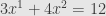
In our matrix notation, this reads

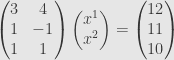
or in purely algebraic notation.

We saw then that this system has no solutions at all. What’s the problem? Well, we’ve got a linear map . The rank-nullity theorem tells us that the dimension of the image (the rank) plus the dimension of the kernel (the nullity) must equal the dimension of the source. But here this dimension is , and so the rank can be at most , which means there must be some vectors which can’t be written as no matter what vector we pick. And the vector in the example is just such a vector outside the image of .

The upshot is that we can only solve the system if the vector lies in the image of the linear map , and it might be less than obvious what vectors satisfy this requirement. Notice that this is more complicated than the old situation for single equations of single variables. In that case, the target only has one dimension, and the linear transformation “multiply by the number ” only misses this dimension if , which is easy to recognize.