Duality terminology

I should have mentioned this before, but usually dual notions are marked by the prefix “co-“. As an example, we have “well-powered” and “co-well-powered” categories.

Another example: We know through Erdős that “a mathematician is a device for turning coffee into theorems”. It thus follows by duality that a comathematician is a device for turning cotheorems into ffee.

The Opposite Category

One of the most interesting general facts about categories is how ubiquitous the notion of duality is. Pretty much everything has a “mirror image”, and the mirror is the opposite category.

Given a category , with objects and morphisms , we can construct the “opposite category” simply enough. In fact, it has the exact same objects and morphisms as does. The difference comes in how they relate to each other.

Remember that we had two functions, and assigning the “source” and “target” objects to any arrow. To get the opposite category we just swap them. Given a morphism, its source in is its target in , and vice versa. Of course, now we have to swap the order of composition. If we have and in , then we get and in . In the composition is defined, but in the composition is defined.

Most definitions we give will automatically come with a “dual” definition, which we get by reversing all the arrows like this. For example, monos and epis are dual notions, as are subobjects and quotient objects. Just write down one definition in terms of morphisms, reverse all the morphisms (and the order of composition), and you get the other.

Theorems work this way too. If you dualize the hypotheses and the conclusions, then you can dualize each step of the proof to prove the dual theorem. I can prove that any injection is monic, so it follows immediately by duality that any surjection is epic. Many texts actually completely omit even the statements of dual notions and theorems once they define the opposite category, but I’ll try to be explicit about the duals (though of course I won’t need to give the proofs).

Another place duality comes up is in defining “contravariant” functors. This is just a functor . It sends each object of to an object of , and sends a morphism in to a morphism in . See how the direction of the image morphism flipped? Early on, contravariant and regular (“covariant”) functors were treated somewhat separately, but really they’re just the same thing once you take the opposite category into account. Sometimes, though, it’s easier to think in terms of contravariant functors rather than mentally flipping all the arrows.

I’ll close with an example of a contravariant functor we’ve seen before. Consider a ring with unit and a left module over . That is, is an object in the category . We can construct the dual module , which is now an object in the category of right -modules. I say that this is a contravariant functor. We’ve specified how the dual module construction behaves on objects, but we need to see how it behaves on morphisms. This is what makes it functorial.

So let’s say we have two left -modules and , and an -module homomorphism . Since we want this to be a contravariant functor we need to find a morphism . But notice that , and similarly for . Then we have the composition of -module homomorphisms . If is a linear functional on , then we get as a linear functional on . We can define .

Now, is this construction functorial? We have to check that it preserves identities and compositions. For identities it’s simple: , so every linear functional on gets sent back to itself. For compositions we have to be careful. The order has to switch around because this is a contravariant functor. We take and and check , as it should.

Solution to the ARML Scrimmage Power Question

Today I’ll give my own solution to the power question I posted last week. I’m going to present it as I always wished I could have: as a whole with answers to the specific questions spun off as they naturally arise, rather than separated part by part.

First I’ll restate the setup into a more natural language. This is really a question about certain endomorphisms on vector spaces over the field . This is the quotient of the ring of integers by the maximal ideal generated by . If you haven’t seen it before, you should be able to construct it by all I’ve said so far.

Anyhow, the “arrangements” are just vectors in the vector space . Such a space comes with a basis , where has a in place and elsewhere. Each of these spaces of course has the identity endomorphism , and it also has a “left rotation” endomorphism sending to and to , and its inverse — right rotation. The transformation we are concerned with is .

Since we are given bases we are justified in writing out matrices for transformations, and even for vectors (because ). The transformation has the matrix where is if or and otherwise. A vector of length will be an matrix.

Numbers 1 and 2 are just calculations, so I’ll omit them.

We can write as the matrix , so has matrix , which sends every vector to the zero vector. This is part 4.

Now one interesting property we can see straight off. We can tell whether there are an even or an odd number of ones in a given arrangement by adding up all the entries. That is, we can take the product with the matrix consisting of all ones. If we first transform an arrangement , then measure the number of ones, this is like taking the product . But each column of the matrix for has exactly two ones in it, so the product consists of all zeroes, and thus is always zero. That is, the image of any arrangement after a transformation always has an even number of ones. That’s number 10.

What arrangements are fixed by the transformation? This amounts to solving the equation

so we must have or . The zero vector is the only fixed point.

What vectors get sent to this fixed point? This is the kernel of the transformation — the vectors such that . Equivalently, these satisfy (why?). Thus all the entries must be the same, and the vector must consist of all zeroes or all ones. That’s number 9.

Now we see that if then is in the kernel of , and is thus either all zeroes or all ones. But if is odd, the vector consisting of all ones is not in the image of . Thus if we don’t start with a vector in the kernel we’ll never land in the kernel, and we’ll never get to the vector of all zeroes. That’s number 11. As a special case we have number 3.

Let’s consider . We expand this as , since we’re working over . Similarly, if we square this we get . In fact, we have that . Indeed, this is true by definition for , and if it’s true for then

so the claim is true by induction.

This means that after transformations a vector is sent to the sum (in ) of itself with its left-rotation by places. Thus if we can divide the entries in into vectors of length each — just pick the entries spaced out by separations of . Then acts on the same way acts on each of the subvectors, since the shift by places fixes the subvectors. That’s number 7. Parts 5 and 6 are now special cases.

Also, if then , so , so transformations send every vector of length to zero. That’s number 8.

Finally, let be any even number that is not a power of . Now the result of is the same as applying to each of the subvectors as described above. But now each subvector has odd length. If has a single in it, then one of these subvectors must contain it. By number 11 this subvector can never be sent to zero, so is never zero. If were ever zero then would be for a large enough , which will never happen. That’s part 12.

Equivalence of categories

It should be pretty clear from all the examples in groups, rings, and modules that two categories and are isomorphic if there are functors and so that is the identity functor on and is the identity functor on .

Unfortunately, that’s not really as useful as it is in more mundane structures. The problem is that isomorphism is really strict, and categories are more naturally sort of loose and free-flowing. We have to weaken the notion of isomorphism to get something really useful. I’ll try to motivate this with one example. It’s sort of simple, but it gets to the heart of the problem pretty quickly.

Remember the category with one object and its identity morphism. We draw it as , taking the identity as given. Let’s also consider a category with two objects and two non-identity morphisms, one going in either direction: . Call the objects and , and the four arrows , , , , where goes from to . Then we have and . That is, the two non-identity arrows are inverses to each other, and the two objects are thus isomorphic.

Now since the two objects in our toy category are isomorphic, they are “essentially the same”. The category should (and does) behave pretty much the same as the category , but they’re clearly not isomorphic as categories.

Here’s another way they’re “the same” category. Since each hom-set in our toy category has at most one object, we can consider it as a preorder. We have the set with and in the order. If we (as usual) move to a partial order, we identify these two points and just get the unique partial order on one point — the category !

Okay, so if they’re not isomorphic, what are they? The key here is that the two objects in our toy category are isomorphic, but not identical. The definition of isomorphism of categories requires that (for example) is exactly again. But really should it matter if we don’t get back itself, but just an object isomorphic to it? Not really. And we also shouldn’t care if we get different results for every object in as long as they’re all isomorphic to the object we stick into , and as long as these isomorphisms all fit together nicely with morphisms between the objects.

The upshot of all this is that we do know how to weaken the concept of isomorphism of categories: we just change the functor equalities in the definition to natural isomorphisms of functors! That is, we have natural isomorphisms and . Let’s unpack this all for our toy category.

The functor from to is the only one possible: send both objects to the single object in and all the arrows to its identity. For a functor the other way we have two choices. Let’s send the singlt object of to the object . The identity arrow must then go to . Now we need natural isomorphisms.

To find these, let’s write down the compositions explicitly: sends the single object of to the object in our toy category, which then gets sent back to the single object in . Its identity arrow just comes along for the ride. Thus is exactly the identity functor on , so we can just use its identity natural transformation as our .

On the other hand, sends both objects of our toy category to the object , and all four arrows to the identity arrow . This is clearly not the identity functor on our category, so we need to find a natural isomorphism. That is, we need to find isomorphisms and so that the two nontrivial naturality squares commute. Clearly we can only pick and . Now if we write out the naturality squares for and (do it!) we see that they do commute, so is a natural isomorphism.

When we have two functors running back and forth between two categories so that their composites are naturally isomorphic to the respective identities like this, we say that they furnish an “equivalence”, and that the categories are “equivalent”. Every isomorphism of categories is clearly an equivalence, but there are many examples of categories which are equivalent but not isomorphic. This is a much more natural notion than isomorphism for saying categories are “essentially the same”.

Special kinds of morphisms, subobjects, and quotient objects

Last week I was using the word “invertible” as if it was perfectly clear. Well, it should be, more or less, since categories are pretty similar to monoids, but I should be a bit more explicit. First, though, there’s a few other kinds of morphisms we should know.

We want to motivate these definitions from what we know of sets, but the catch is that sets are actually pretty special. Some properties turn out to be the same when applied to sets, though they can be different in other categories.

First of all, let’s look at injective functions. Remember that these are functions where implies . That is, distinct inputs produce distinct outputs. Now we can build a function as follows: if for some we define . This is well-defined because at most one can work, by injectivity. Then for all the other elements of we just assign them to random elements of . Now the composition is the identity function on because for all . We say that the function has a (non-unique) “left inverse”.

Now since has a left inverse there’s something else that happens: if we have two functions and both from to , and if then . That is, is “left cancellable”.

Now in any category we say a morphism is a “monomorphism” (or “a mono”, or “ is monic”) if it is left cancellable, whether or not the cancellation comes from a left inverse as above. If has a left inverse we say is “injective” or that it is “an injection”. By the same argument as above, every injection is monic, but in general not all monos are injective. In the two concepts are the same.

Similarly, a surjective function has a right inverse , and is thus right cancellable. We say in general that a right cancellable morphism is an “epimorphism” (or “an epi”, or “ is epic”). If the right cancellation comes from a right inverse, we say that is “surjective”, or that it is “a surjection”. Again, every surjection is epic, but not all epis are surjective. In the two concepts are again the same.

If a morphism is both monic and epic then we call it a “bimorphism”, and it can be cancelled from either side. If it is both injective and surjective we call it an “isomorphism”. All isomorphisms are bimorphisms, but not all bimorphisms are isomorphisms. If is an isomorphism, then we can show (try it) that the left and right inverses are not only unique, but are the same, and we call the (left and right) inverse . When I said “invertible” last week I meant that such an inverse exists.

We’ve already seen these terms in other categories. In groups and rings we have monomorphisms and epimorphisms, which are monos and epis in the categories and .

Now recall that any subset of a set comes with an injective function “including” into . Similarly, subgroups and subrings come with “inclusion” monomorphisms. We generalize this concept and define a “subobject” of an object in a category to be a monomorphism . In the same way we generalize quotient groups and quotient rings by defining a “quotient objects” of to be epimorphisms .

Notice that we define a subobject to be an arrow, and we allow any monomorphism. Consider the function defined by and . It seems odd at first, but we say that this is a subobject of . The important thing here is that we don’t define these concepts in terms of elements of sets, but in terms of arrows and their relations to each other. We “can’t tell the difference” between and since they are isomorphic as sets. If we just look at the arrow and the usual inclusion arrow of , they pick out the same subset of so we may as well consider them to be the same subset.

Let’s be a little more general here. Let and be two subobjects of . We say that “factors through” if there is an arrow so that . If we take the class of all subobjects of (all monomorphisms into ) we can give it the structure of a preorder by saying if factors through . It should be straightforward to verify that this is a preorder.

Now we can turn this preorder into a partial order as usual by identifying any two subobjects which factor through each other. If and then . Since is monic we can cancel it from the left and find that . similarly we find that . That is, and are inverses of each other, and so and are isomorphic as subobjects of . Conversely, if and are isomorphic subobjects then and factor through each other by an isomorphism . This gives us a partial order on (equivalence classes of) subobjects of . If the class of equivalence classes of subobjects is in fact a proper set for every object we say that our category is “well-powered”.

The preceding two paragraphs can be restated in terms of quotient objects. Just switch the directions of all the arrows and the orders of all the compositions. We get a partial order on (equivalence classes of) quotient objects of . If the class of equivalence classes is a proper set for each object then we say that the category is “co-well-powered”.

It should be noted that even though isomorphic subobjects come with an isomorphism between their objects, just having an isomorphism between the objects is not enough. One toy example is given in the comments below. Another is to consider two distinct one-element subsets of a given set. Clearly the object for each is a singleton, and all singletons are isomorphic, but the two subsets are not isomorphic as subobjects.

As an exercise, consider the category of commutative rings with unit and determine the partial order on the set of quotient objects of .

New This Week’s Finds

Now, back to the math. John Baez has posted a new This Week’s Finds. He continues his “Tale of Groupoidification”. It features a great comparison of group actions on sets and those on vector spaces (which we’ll get to soon enough). Even better, he gives a translation “for students trying to learn a little basic category theory” into the language of categories.

Natural Transformations and Functor Categories

So we know about categories and functors describing transformations between categories. Now we come to transformations between functors — natural transformations.

This is really what category theory was originally invented for, and the terminology predates the theory. Certain homomorphisms were called “natural”, but there really wasn’t a good notion of what “natural” meant. In the process of trying to flesh that out it became clear that we were really talking about transformations between the values of two different constructions from the same source, and those constructions became functors. Then in order to rigorously define what a functor was, categories were introduced.

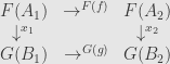
Given two functors and , a natural transformation is a collection of arrows in indexed by the objects of . The condition of naturality is that the following square commutes for every arrow in :

The vertical arrows from from applying the two functors to the arrow , and the horizontal arrows are the components of the natural transformation.

If we have three functors , , and from to and natural transformations and we get a natural transformation with components . Indeed, we can just stack the naturality squares beside each other:

and the outer square commutes because both the inner ones do.

Every functor comes with the identity natural transformation , whose components are all identity morphisms. Clearly it acts as the identity for the above composition of natural transformations.

A natural transformation is invertible for the above composition if and only if each component is invertible as an arrow in . In this case we call it a “natural isomorphism”. We say two functors are “naturally isomorphic” if there is a natural isomorphism between them.

All of this certainly looks like we’re talking about a category, but again the set theoretic constraints often work against us. There are, however, times where we really do have a category. If one of or (or both) are small, then all the set theory works out and we get an honest category of functors from to . We will usually denote this category as . Its objects are functors from to , and its morphisms are natural transformations between such functors.

And now we can explain the notation for the category of arrows. This is the category of functors from to ! What is a functor from to ? Remember that is the category with two objects and and one non-trivial arrow . Thus a functor is defined by an arrow , and there’s exactly one functor for every arrow in .

Now let’s say we have two such functors and . A natural transformation consists of morphisms and so that the naturality square commutes. But this is the same thing we used to define morphisms in the arrow category, just with some different notation!

Natural transformations and functor categories show up absolutely everywhere once you know to look for them. We’ll be seeing a lot more examples as we go on.

Comma Categories

Another useful example of a category is a comma category. The term comes from the original notation which has since fallen out of favor because, as Saunders MacLane put it, “the comma is already overworked”.

We start with three categories , , and , and two functors and . The objects of the comma category are triples where is an object of , is an object of , and is an arrow in . The morphisms are pairs — with an arrow in and an arrow in — making the following square commute:

So what? Well, let’s try picking to be the functor sending the single object of to the object . Then let be the identity functor on . Now an object of is an arrow , where can be any other object in . A morphism is then a triangle:

Work out for yourself the category .

Here’s another example: the category . Verify that this is exactly the arrow category .

And another: check that given objects and in , the category is the discrete category (set) .

Neat!

Ave, Borcherds

I know I’m a few days late in this, but I’d like to extend a welcome to Richard Borcherds, newest blatherer.

Cardinals and Ordinals as Categories

We can import all of what we’ve said about cardinal numbers and ordinal numbers into categories.

For cardinals, it’s actually not that interesting. Remember that every cardinal number is just an equivalence class of sets under bijection. So, given a cardinal number we can choose a representative set and turn it into a category . We let and just give every object its identity morphism — there are no other morphisms at all in this category. We call this sort of thing a “discrete category”.

For ordinal numbers it gets a little more interesting. First, remember that a preorder is a category with objects the elements of the preorder, one morphism from to if , and no morphisms otherwise.

It turns out that (small) categories like this are exactly the preorders. Let be a small category with a set of objects and no more than one morphism between any two objects. We define a preorder relation by saying if is nonempty. The existence of identities shows that , and the composition shows that if and then , so this really is a preorder.

If now we require that no morphism (other than the identity) has an inverse, we get a partial order. Indeed, if and then we have arrows and . We compose these to get and . These must be the respective identities because there’s only the one arrow from any object to itself. But we’re also requiring that no non-identity morphism be invertible, so has to be the same object as .

Now we add to this that for every distinct pair of objects either or is nonempty. They can’t both be — that would lead to an inverse — but we insist that one of them is. Here we have total orders, where either or .

Finally, a technical condition I haven’t completely defined (but I will soon): we require that every nonempty “full subcategory” of have an “initial object”. This is the translation of the “well-ordered” criterion into the language of categories. Categories satisfying all of these conditions are the same as well-ordered sets.

Okay, that got a bit out there. We can turn back from the theory and actually get our hands on some finite ordinals. Remember that every finite ordinal number is determined up to isomorphism by its cardinality, so we just need to give definititions suitable for each natural number.

We define the category to have no objects and no morphisms. Easy.

We define the category to have a single object and its identity morphism. If we take the identity morphisms as given we can draw it like this: .

We define the category to have two objects and their identity morphisms as well as an arrow from one object to the other (but not another arrow back the other way). Again taking identities as given we get .

Things start to get interesting at . This category has three objects and three (non-identity) morphisms. We can draw it like this:

The composite of the horizontal and vertical arrows is the diagonal arrow.

Try now for yourself drawing out the next few ordinal numbers as categories. Most people get by without thinking of them too much, but it’s helpful to have them at hand for certain purposes. In fact, we’ve already used !

Now to be sure that this does eventually cover all natural numbers. We can take our to be the category . Then for a successor “function” we can take any category and add a new object, its identity morphism, and a morphism from every old object to the new one. With a little thought this is the translation into categories of the proof that well-ordered finite sets give a model of the natural numbers, and the same proof holds true here.