We’ve actually already seen the  root system, back when we saw a bunch of two-dimensional root system. But let’s examine how we can construct it in line with our setup.
The root system is, as we can see by looking at it, closely related to the  root system. And so we start again with the
  -dimensional subspace of
  consisting of vectors with coefficients summing to zero, and we use the same lattice
  . But now we let
  be the vectors
  of squared-length or
  :
:  or
or  . Explicitly, we have the six vectors from —
  ,
,  , and
, and  — and six new vectors —
 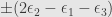 ,
, 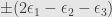 , and
, and  .
.
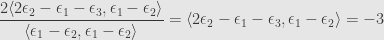
We can pick a base  . These vectors are clearly independent. We can easily write each of the above vectors with a positive sign as a positive sum of the two vectors in
  . For example, in accordance with an earlier lemma, we can write

where after adding each term we have one of the positive roots. In fact, this path hits all but one of the six positive roots on its way to the unique maximal root.
It’s straightforward to calculate the Cartan integers for .

which shows that we do indeed get the Dynkin diagram .
And, of course, we must consider the reflections with respect to both vectors in . Unfortunately, computations like those we’ve used before get complicated. However, we can just go back to the picture that we drew before (and that I linked to at the top of this post). It’s a nice, clean, two-dimensional picture, and it’s clear that these reflections send back to itself, which establishes that is really a root system.
We can also figure out the Weyl group geometrically from this picture. Draw line segments connecting the tips of either the long or the short roots, and we find a regular hexagon. Then the reflections with respect to the roots generate the symmetry group of this shape. The twelve roots are the twelve axes of symmetry of the polygon, and we can get rotations by first reflecting across one root and then across another. For example, rotating by a sixth of a turn can be effected by reflecting with the basic short root, followed by reflecting with the basic long root.
Finally, we can see that this root system is isomorphic to its own dual. Indeed, if  is a short root, then the dual root is itself:

On the other hand, if is a long root, then we find

and so the squared-length of  is
is  . These are now the short roots of the dual system. Scaling the dual system up by a factor of
  and rotating
  of a turn, we recover the original root system.
March 8, 2010
Posted by John Armstrong |
Geometry, Root Systems |
1 Comment

